Section 1: Why We Need Regularization
Where we left off
Last lecture we saw that weight sharing and sparse connectivity tame the parameter explosion of fully-connected layers, and that backprop through a convolution is itself a convolution (with the kernel flipped). But the punchline was: CNNs can still overfit, even though they have far fewer parameters than an equivalent fully-connected layer. So today’s question is: what should we do about overfitting?
Regularization is one tool among many
Regularization is one strategy to improve generalization, and it is just one of many ways to do it. The boundary between regularization and other engineering techniques is not always clear. A rough way to think about the whole pipeline is:
- Dataset
- Architecture setup
- Normalization
- Training loop
- Regularization
The general strategies against overfitting are:
- Collect more data, especially high-quality data. This is the best option and always recommended (semi-supervised learning, transfer learning and self-supervised learning are ways to get more out of the data we have).
- Data augmentation is helpful.
- Reducing model capacity can help.
Note that training is basically maximum likelihood, so the model is only ever as good as the data it is fit on. That is why high-quality data comes first. Which of the other tools is best is “not entirely settled”, and it depends on the problem.
The bias-variance trade-off
For regression with squared-error loss, the expected prediction error at a fixed input
- Bias is the error from a model that is too simple to capture the true pattern.
- Variance is the error from a model that is too sensitive to the specific training sample it happened to see.
Increasing capacity (more layers or units) typically lowers bias but raises variance. This gives us a useful way to look at every regularizer in this lecture: each technique trades a little bias for a lot less variance.
The accuracy example below illustrates underfitting and overfitting qualitatively. The squared-error identity above does not decompose classification accuracy into these three terms.
| Model | Train acc. | Test acc. | Diagnosis |
|---|---|---|---|
| A: small MLP | 60% | 58% | Both low, so high bias (underfitting) |
| B: large MLP | 99% | 71% | Huge gap, so high variance (overfitting) |
Model B is actually the better model, even though it overfits. A large model that we then regularize usually beats starting with a small one.
Rule of thumb: if the training accuracy is low, look at bias. If the train/test gap is big, look at variance.
This is why the advice was: first overfit a model, then regularize it, instead of starting with a smaller model and hoping it is the right size.
Section 2: More Data and Data Augmentation
More data is the cleanest way to reduce variance. Data is valuable, but often we cannot afford more of it. Data augmentation is the cheap alternative.
The idea: if we know the label should not depend on some transformation
The catch is that we must already know something our outcome does not depend on. For image classification, the label should not change under, e.g., rotation, zooming or a sepia filter. But a transformation that changes the label is harmful. For digit recognition, flipping a “6” by 180° turns it into a “9”
In PyTorch this is done with TorchVision. The lecture example uses MNIST: the randomly augmented digits are slightly cropped and rotated versions of the originals, but still show the same digit, so the label stays the same. The key detail is that random augmentation is applied only to the training data. The test transform is deterministic (resize, then crop the center), so that the evaluation is reproducible:
The two pipelines differ in exactly the random steps (RandomCrop, RandomRotation in training and CenterCrop at test time), while the final normalization to L10/code/data-augmentation.ipynb in the repository rasbt/stat453-deep-learning-ss21.
Section 3: Reducing Capacity and Early Stopping
The simplest model that fits should generalize best
Several knobs shrink the effective capacity of a network:
- Smaller architecture: fewer hidden layers and units.
- Smaller weights: early stopping, L2 norm penalty.
- Sparse weights or activations: ReLU with an L1 penalty prunes units.
- Noise: dropout.
For recent LLMs and foundation models there is another option: take a large pretrained model and do efficient fine-tuning. We freeze most of the weights and only train (fine-tune) the remaining small number of parameters.
Three data splits
Early stopping needs us to be careful with the data splits. As always we split into three parts:
- Training set: used to update the weights.
- Validation set: used for tuning (hyperparameters, when to stop). It lives inside the training loop.
- Test set: used once at the end, outside the loop. In the end we care about the test accuracy, so we must not touch it before.
Some fields swap the names of test and validation (medicine, for example), so watch the terminology when reading papers.
Early stopping
Track a validation metric during training and keep the checkpoint that scores best on that metric.
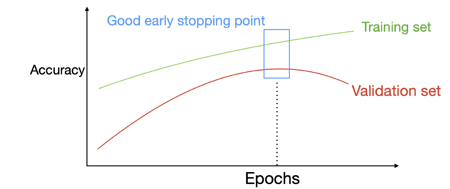
In practice we keep a copy of the best weights seen so far and stop once the validation performance has not improved for a number of epochs, called the patience. The code below monitors the validation loss, where lower is better. The figure above plots accuracy, where higher is better, so if you monitor accuracy instead, just flip the comparison (val_acc > best_val) and start from -inf:
Early stopping acts as an implicit regularizer by restricting the selected parameters to checkpoints along the training trajectory. If validation performance deteriorates while training performance improves, restoring an earlier checkpoint can improve generalization.
For linear least squares with zero initialization and a stable step size, early stopping and ridge regression both suppress directions of low curvature. In this setting,
Section 4: Norm Penalties (L1 and L2)
Adding a penalty to the loss
We add a penalty on the size of the weights to the loss:
where
- L2 penalizes
\Omega(w)=\sum_i w_i^2 . This is the same idea as ridge regression, and it encourages small values. - L1 penalizes
\Omega(w)=\sum_i \lvert w_i \rvert . This is the same idea as LASSO, and it encourages zeros, i.e. sparse solutions.
In neural networks we typically only penalize the weights and leave the biases alone
Regularization is MAP estimation
In Lecture 3 we saw that MAP estimation with a Gaussian prior gives L2 and with a Laplace prior gives L1. Here is the derivation again. MAP maximizes the posterior
So the penalty is nothing but the negative log of the prior:
| Prior |
Penalty | Name |
|---|---|---|
| Gaussian | L2 / ridge | |
| Laplace | L1 / LASSO |
Geometric picture
Penalizing the norm is the same as constraining the weights to lie in a region around the origin: a circle (ball) for L2 and a diamond (square rotated by 45°) for L1. The solution is the point where the contours of the data loss first touch the region.
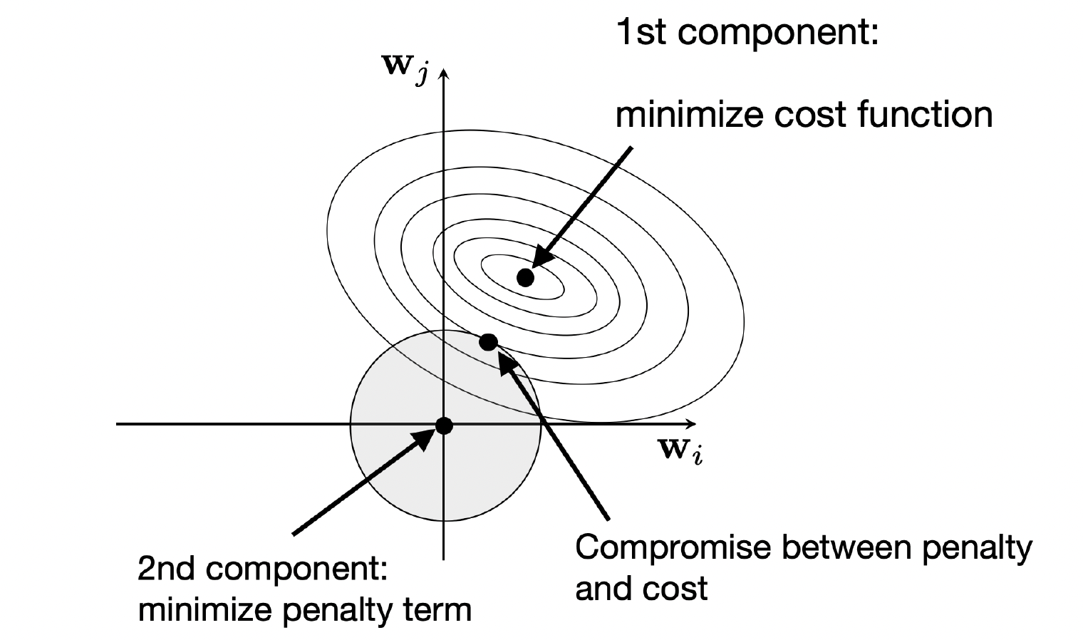
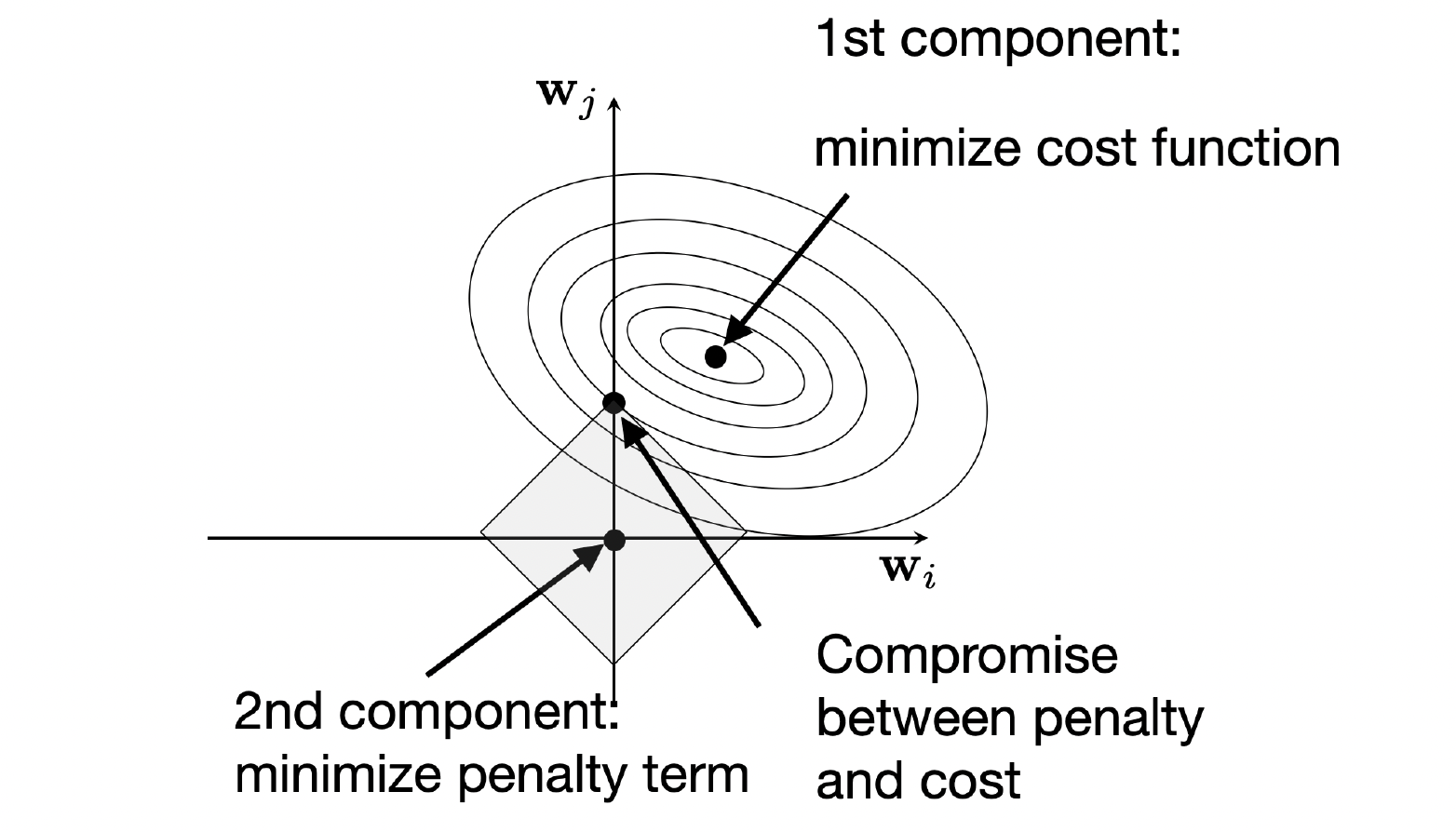
The corners of the diamond lie on the axes, and that is why L1 produces sparse solutions while L2 only shrinks.
Weight decay
For multilayer networks we simply sum the penalty over all layers. In the notation of the lecture, with
where
Rewriting the right-hand side gives
L2 regularization in PyTorch
In PyTorch you can add the penalty to the cost manually, or let the optimizer do it with weight_decay:
The parameter groups apply weight decay only to parameters whose names contain ‘weight’. Biases remain trainable but receive no weight decay, matching the weight-only policy in the manual example above.
weight_decay=LAMBDA, SGD adds LAMBDA * w to the gradient, so LAMBDA plays the role of the factor in front of w in the update above. For adaptive optimizers like Adam this is not exactly the same as an L2 penalty, which is why AdamW exists.======= The factor of two comes from differentiating the squared norm. Both alternatives apply the same gradient to the same weights. Use one option per update to avoid applying the penalty twice. AdamW decouples parameter shrinkage from the adaptive gradient update, so its weight decay differs from adding an L2 penalty to Adam’s loss.
Section 5: Dropout
Dropout is a deep-learning-specific method. When propagating forward during training, we randomly drop some neurons by setting their activations to 0.
Bernoulli masks
With drop probability
In practice we sample
Why does it work?
- No single connection can be relied on. The network cannot depend on particular connections too heavily, so it has to use more of them. The weights end up more spread out, which may lead to smaller weights, similar to the L2 norm. (As a side note from the slides: you can use different dropout probabilities in different layers, and assigning them proportional to the number of units in a layer is not a bad idea.)
- Implicit ensemble. Every minibatch trains a different sub-network. With
h hidden units there areM = 2^h possible masks, so over the minibatch iterations we sample from an exponentially large family of models. These models share weights, which is itself a form of regularization. At inference time we could average over all of these models, but that is extremely expensive. This is where the trick below comes in.Goodfellow et al. describe dropout as making bagging practical for exponentially many large networks. - It suppresses high-order interactions. This is the view from the lecturer’s own paper on dropout and interaction effects
. An interaction of order k is an effect that needsk variables at the same time (e.g. “feature A and feature B together”). Two things happen ask grows:- With
N input variables there are\binom{N}{k} possible order-k interactions, which grows roughly likeN^k for the first few orders. So there are many more high-order combinations that could fit noise in the training data. - An order-
k interaction only survives a dropout step if allk of its variables survive. With drop rater this has probability(1-r)^k , which decays exponentially ink .
The slide then states that these exponential rates cancel out, and that this anti-interaction regularization happens at every layer.
The slide only has this one line about the cancellation. One way to read it is that the exponentially growing number of candidate interactions and the exponentially decaying survival probability work against each other, so it is not obvious in advance which one wins. The paper is what shows that the net effect is a suppression of higher orders. The net effect is that dropout puts more pressure on higher-order effects than on low-order ones. In the experiment from the paper that is shown on the slide, the share of the normalized effect size that comes from first-order (additive) terms grows from roughly a quarter to roughly three quarters when the dropout rate goes from 0 to 0.75, while the higher orders shrink. A practical consequence: if you want to regularize away more complex interactions, increase the dropout rate. - With
Inverted dropout and train() vs. eval()
If we drop units during training but use all units at test time, the expected input to the next layer changes. The fix is inverted dropout: scale the surviving activations by
For a keep probability
In PyTorch the behavior depends on the mode of the model:
model.train()turns dropout on. Use this in the training loop.model.eval()turns dropout off. Use this when you just want to see how good the model is.
Forgetting model.eval() is a classic bug: the validation numbers come out noisy and too pessimistic, because dropout is still active.
The slides compare training with and without dropout on MNIST with a multilayer perceptron. Without dropout, the training accuracy goes towards 100% while the validation accuracy plateaus at around 97 to 98%, so there is a visible gap. With 50% dropout, the training and validation curves lie almost on top of each other at roughly 97.5%, so the gap is gone. The minibatch loss is noisier and stays higher, because every step uses a randomly thinned network.
Key Takeaways
- The bias–variance decomposition above applies to squared error. Regularization can reduce variance at the cost of higher bias.
- Low training accuracy can flag underfitting or an optimization problem. A large training–validation gap can flag overfitting.
- More (and more diverse) data is the best fix. Augmentation only helps if we know a transformation the label does not depend on, and it is applied only to the training data.
- Early stopping uses the validation set to pick the stopping point and acts as an implicit regularizer. The test set is touched only once.
- L2 (ridge, Gaussian prior) encourages small weights. L1 (LASSO, Laplace prior) encourages zeros. Both are just the negative log of a prior added to the data loss.
- Dropout randomly zeroes units during training, which prevents co-adaptation and approximates averaging over an exponential ensemble of weight-sharing networks. Use
model.train()andmodel.eval()correctly.