Lecture 05: Parameter Optimization and Gradient Descent
From the perceptron's hard threshold to a smooth sigmoid unit, maximum likelihood, stochastic gradient descent, and backpropagation on computation graphs.
1. Today’s Roadmap
- Perceptron
- Soft threshold
\rightarrow likelihood - Gradient descent
- Backpropagation and computation graphs
The thread running through all four: a hard threshold gives us no way to learn from data, so we swap in a smooth activation function, turn the model into a likelihood we can maximize, and then walk up that likelihood with gradient descent. Applying gradient descent to a deep model is backpropagation.
2. Review of the Perceptron from Last Class
2.1 McCulloch and Pitts’ neuron model (1943)
McCulloch and Pitts made a neuron model that had inputs feeding a linear combiner, which passes through a hard limiter to produce an output.
2.2 Rosenblatt’s perceptron (1957)
Rosenblatt built on this by creating the perceptron, which added continuous weighting and an activation (threshold) function.
where
2.3 The perceptron learning algorithm
The algorithm assumes a binary classification task, and it finds a decision boundary if the classes are separable. For a dataset
the pseudocode is:
- Initialize
\mathbf{w} := \mathbf{0}^m (assume the weight vector includes the bias). - For every training epoch:
- For every
\langle \mathbf{x}^{[i]}, y^{[i]} \rangle \in \mathcal{D} :-
\hat{y}^{[i]} := \sigma\left(\mathbf{x}^{[i]T}\mathbf{w}\right) , which is only 0 or 1
-
\textit{err} := \left(y^{[i]} - \hat{y}^{[i]}\right) , which is only
-1 , 0, or 1 -
\mathbf{w} := \mathbf{w} + \textit{err} \times \mathbf{x}^{[i]}
-
- For every
Because the error can only be
2.4 Geometric intuition
The weight vector is perpendicular to the decision boundary. To see why, recall that
At the boundary
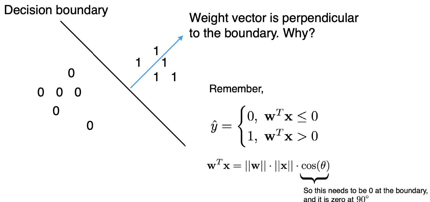
When a point with label 1 lands on the wrong side, we add its input vector to the weight vector. The new weight vector is rotated toward that example, which puts it on the correct side.
3. Beyond Rosenblatt’s Perceptron: Choosing an Activation Function
With a hard threshold function we need some way to learn from data, and the threshold gives us no gradient to work with. Everything beyond the classic perceptron comes from swapping out the activation function:
| Activation function | What the unit becomes |
|---|---|
| Threshold function (perceptron, 1950+) | Classic Rosenblatt perceptron |
| Sigmoid function (before 2000) | Deep learning “perceptron” / sigmoid unit |
| Identity | Linear regression |
| ReLU (popular since CNNs), plus variants such as leaky ReLU and GeLU | Modern deep networks |
If we swap out the activation function for something smooth like the sigmoid, we get a deep learning perceptron, or sigmoid unit. If we use the identity as the activation function we get linear regression.
In lecture. Depth only buys us something when the activation is nonlinear. Stacking units with identity activations composes linear maps into one linear map, so the stack collapses back to a single linear model. Nonlinear activations are what let a stack of units represent functions a single unit cannot.
Making the activation function smooth is the key move. Once it is differentiable, we can apply gradient descent, and applying gradient descent to a deep learning model is backpropagation.
4. The Sigmoid Unit: Logistic Regression Gives Us an Optimizer
4.1 The forward pass
For binary classes
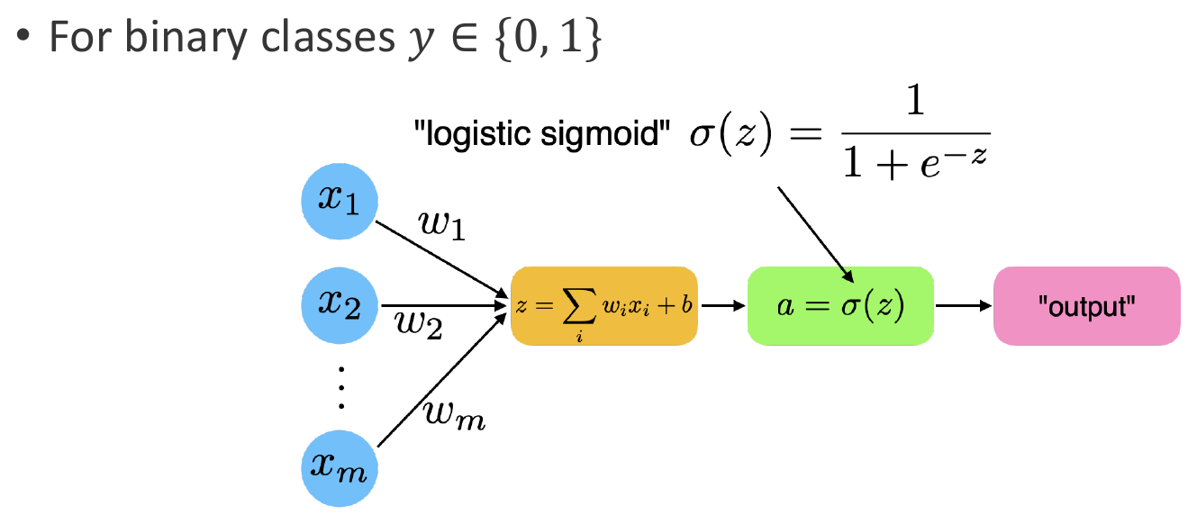
4.2 A probabilistic model
Because the output lies in
Recalling the Bernoulli distribution, the two cases collapse into one expression:
Once we have a probabilistic model we have a likelihood function, and we can optimize it in different ways. Optimizing it by gradient descent is what gives us backpropagation.
4.3 Likelihood and log-likelihood
Under MLE we would like to maximize the multi-sample likelihood:
Since we are going to optimize via gradient descent, we apply the logarithm to separate the components. The maximizer of the likelihood is also the maximizer of the log-likelihood, so nothing is lost:
The log turns a product into a sum, which makes the derivative of each component much easier to compute.
4.4 Deriving the gradient piece by piece
Dividing the equation into parts makes deriving each part easier. By the chain rule,
and the three pieces are
Multiplying them through, the messy denominator cancels:
In lecture. If the post-activation value is very far away from the target, we make a bigger update to our weight. If it is very close, we make a very little weight update. The perceptron could not do this, since its error was only
5. Gradient Descent
5.1 Why we take steps instead of solving
If we want the best weights for our data, we want to maximize the likelihood. If we could set the derivative to zero and solve, we would, but for most deep learning functions we can’t. Instead we take steps in the direction of the gradient (the slope) to reach a local maximum. We can’t guarantee a global maximum, but we can find a local one by walking up the gradient.
So the recipe is: take the derivative first, then walk up the gradient to find the maximizer.
5.2 Stochastic gradient descent
Stochastic gradient descent is a greedy algorithm. At each point it takes one step in the direction that moves us best toward the goal. The gradient tells us which direction to move in, and the weight vector is updated by some step size times that gradient.
- Initialize
\mathbf{w} := \mathbf{0} \in \mathbb{R}^m ,b := 0 . - For every training epoch:
- For every
\langle \mathbf{x}^{[i]}, y^{[i]} \rangle \in \mathcal{D} :- (a)
\hat{y}^{[i]} := \sigma\left(\mathbf{x}^{[i]T}\mathbf{w} + b\right) - (b)
\nabla_{\mathbf{w}}\mathcal{L} = -\left(y^{[i]} - \hat{y}^{[i]}\right)\mathbf{x}^{[i]} and\nabla_{b}\mathcal{L} = -\left(y^{[i]} - \hat{y}^{[i]}\right) - (c)
\mathbf{w} := \mathbf{w} + \eta \times \left(-\nabla_{\mathbf{w}}\mathcal{L}\right) andb := b + \eta \times \left(-\nabla_{b}\mathcal{L}\right)
- (a)
- For every
Here
Using the negative versus the positive gradient is what changes whether we are descending or ascending. We iteratively take steps in the direction of the gradient, which is the slope, and that steps us toward the optimum in a greedy fashion.
6. Multilayer Perceptron
Gradient descent applies to large models too, not just a single unit. A multilayer perceptron is a computation graph with multiple fully-connected layers, and stacking layers allows us to model more functions than a single unit can.
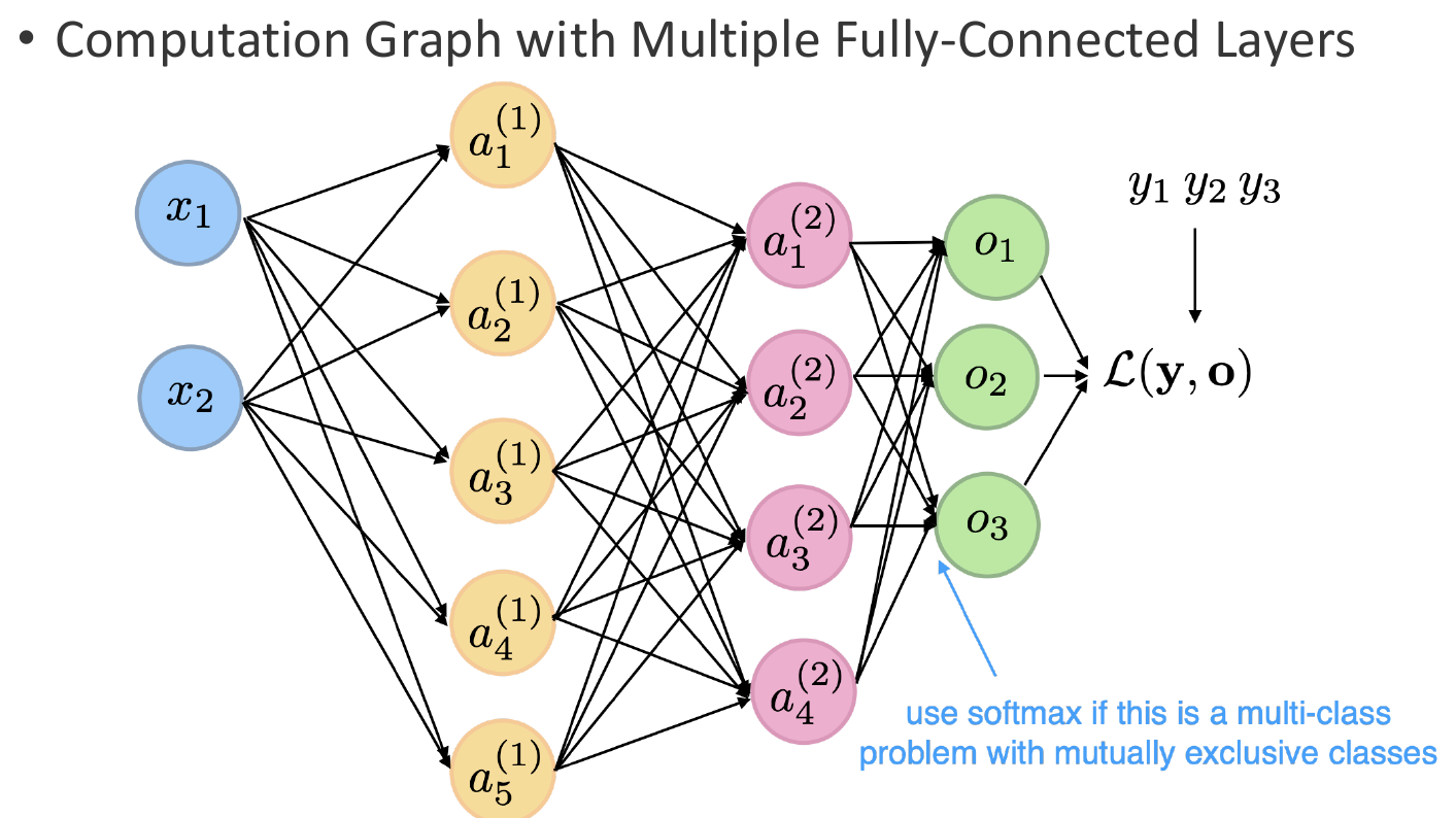
Use softmax at the output if this is a multi-class problem with mutually exclusive classes.
7. Backpropagation and Computation Graphs
7.1 The chain rule is the whole thing
The chain rule is basically the essence of training deep neural networks, and it is the basis for all neural networks and deep learning. For a nested function decomposed into an inner and an outer part,
Neural networks are function compositions that can be represented as computation graphs. By applying the chain rule and working in reverse order, we get
where
7.2 Quick calculus refresher
The derivative of a function is its rate of change, or its slope:
Conceptually we are approximating the slope (the tangent) by a secant between two points and then shrinking the gap. Two worked examples from lecture: for
The rules we lean on are the standard ones: sum, difference, product, quotient, reciprocal, and above all the chain rule,
7.3 PyTorch does this automatically
PyTorch can usually do all of this automatically for us. It literally keeps a computation graph in the background, so when you define
7.4 Worked example: ReLU
ReLU is the Rectified Linear Unit, probably the most commonly used activation function in deep learning. Every input that is positive is sent straight to the output, and every input that is negative is set to 0:
Take the activation
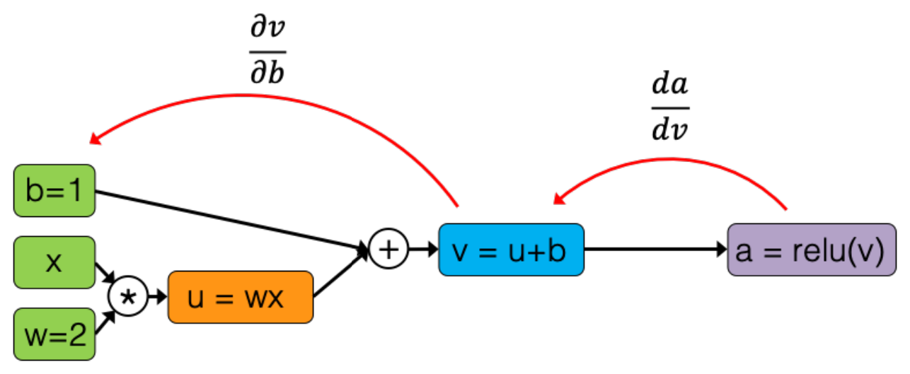
Then we can work backwards with the chain rule, doing
7.5 Single-path graphs
For a single path, we take the product of each of these derivatives, which is the univariate chain rule. For
7.6 Fully-connected layers
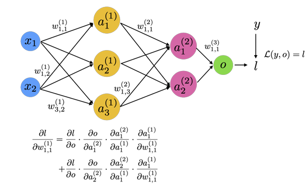
For a fully-connected layer we have to sum the different paths of derivatives from the input weight to the output, because a single weight influences the loss through every downstream unit it feeds. Backprop traces how much a weight affects the output using the chain rule along each of those paths:
7.7 Weight sharing
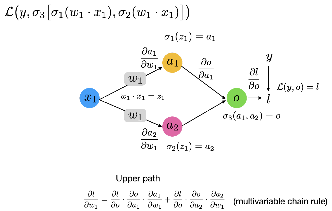
Weight sharing happens in convolutional neural networks. CNNs are really good for image recognition because a fully-connected network would not work at that scale, since that is far too many paths connecting every pixel to every other pixel. So CNNs reuse the same weight in many places, and it works really well.
When weights are shared across different paths, we have to use the multivariable chain rule and sum up the contributions of each of the paths the shared weight appears on. For
8. Summary
- The perceptron adds continuous weighting and an activation function to the MP neuron.
- Its update just adds or subtracts the input vector, because the error is only
-1 , 0, or 1. - The weight vector is perpendicular to the decision boundary.
- The activation function decides what the unit is: threshold gives the perceptron, identity gives linear regression, sigmoid gives the sigmoid unit, and ReLU is the modern default.
- A smooth activation is differentiable, which is what lets us use gradient descent.
- The sigmoid unit is a Bernoulli model, so we can write a likelihood and maximize it.
- Taking the log turns the product into a sum and makes each derivative easy.
- The gradient works out to
(a - y)x_j , so predictions far from the target give big updates and close ones give small updates. - SGD is greedy. It takes one step at a time in the direction the gradient points, scaled by the learning rate.
- Backpropagation is the chain rule applied in reverse over a computation graph.
- One path means multiplying the derivatives. Several paths means multiplying along each one and adding them up.