Lecture 07: Multi-layer Perceptrons and Backpropagation
From binary to multi-class classification with softmax, stacking fully-connected layers into a multi-layer perceptron, the nonlinear activations that finally solve XOR, and backpropagation in matrix form.
Section 1: From Binary to Multi-Class Classification
Moving from Two Classes to K Classes
Binary classification (2 categories). When deciding between just two things — “spam” or “not spam” — we use the sigmoid, which squashes the network’s output into a probability between 0 and 1. This is the setup from Lecture 6:
Multi-class classification (K categories). With multiple categories, the model outputs a raw, unnormalized score — a logit — for every category, and the label follows a categorical distribution:
The Softmax Function
We need a way to turn those raw scores into probabilities. Softmax is a fixed mathematical rule — it has no trainable parameters, so it does not “learn” — that makes every score positive with an exponential and divides by the total, so the outputs lie between 0 and 1 and sum to exactly 1:
The sigmoid is exactly the
From Likelihood to Cross-Entropy Loss
Likelihood. This measures the probability the model assigned to the correct answer.
When the label is a one-hot vector such as
Taking logs turns that product into a sum:
Cross-entropy loss. To train the model we want a loss that goes down as the model gets better, so we take the negative log-likelihood:
This is the categorical cross-entropy, and it is the same recipe as Lecture 6 with more
classes. In PyTorch, nn.CrossEntropyLoss takes the raw logits directly, just as
BCEWithLogitsLoss did — the softmax is applied internally for numerical stability, so
you should not apply it yourself first.
The Gradient: Same Pattern, More Classes
To fix its errors, the network needs to know how to adjust its raw scores. Softmax
combined with cross-entropy has a simple closed-form gradient, elementwise in
This is the same
Section 2: Multi-layer Perceptron Architecture
Stacking Fully-Connected Layers
An MLP is a computation graph built from multiple fully-connected layers, and as the lecture puts it, there is “nothing new, really” in the individual pieces: each layer is the same affine map followed by an activation that we have seen since Lecture 4. What is new is that the output of one layer becomes the input of the next.
If a network only uses straight-line math, it cannot solve complex, overlapping patterns such as the famous XOR problem. We must introduce bends and curves into the math using nonlinear activation functions such as ReLU — which is what Section 3 takes up in detail.
Counting the Trainable Parameters
A question worth answering carefully, because it recurs every time you design a network:
how many trainable parameters does an MLP actually have? For a fully-connected layer
mapping
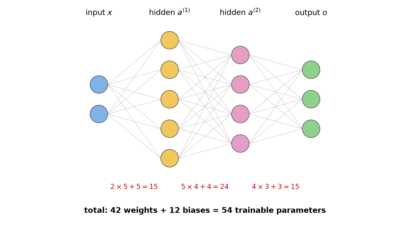
Applying that rule layer by layer to the network above:
| Layer | Weights | Biases | Total |
|---|---|---|---|
| Layer 1 ( |
5 | 15 | |
| Layer 2 ( |
4 | 24 | |
| Layer 3 ( |
3 | 15 | |
| Total | 42 | 12 | 54 |
So the network has 54 trainable parameters. Note also that because the three outputs are mutually exclusive classes, this is a multi-class problem and the output layer uses the softmax of Section 1.
Updating the Early Layers
Counting parameters raises the obvious follow-up: how does a weight in the first layer get updated, when it only affects the loss indirectly? The network has to account for every path along which that weight influences the final prediction, multiplying the local derivatives backward through the network with the chain rule and summing over paths. Section 4 makes that statement precise and shows that “sum over paths” is exactly a matrix multiplication.
Section 3: Nonlinear Activation Functions
Why Stacking Layers Is Not Enough
Section 2 stacked fully-connected layers into a computation graph, but stacking alone buys us nothing. Consider two linear layers with no activation between them:
The composition collapses back into a single linear map. A hundred such layers is still one linear layer with a more expensive parameterization, so the decision boundary is still a single hyperplane — exactly the limitation that the perceptron ran into.
XOR makes the failure concrete. The four clusters alternate labels along both axes, so
no single line separates them. Training a one-hidden-layer MLP with the identity
activation produces exactly one straight boundary and misclassifies half the data.
Swapping the identity for ReLU on the same architecture produces a piecewise-linear
boundary that bends around the clusters and separates them. The nonlinearity, not the
depth, is what buys the expressiveness.
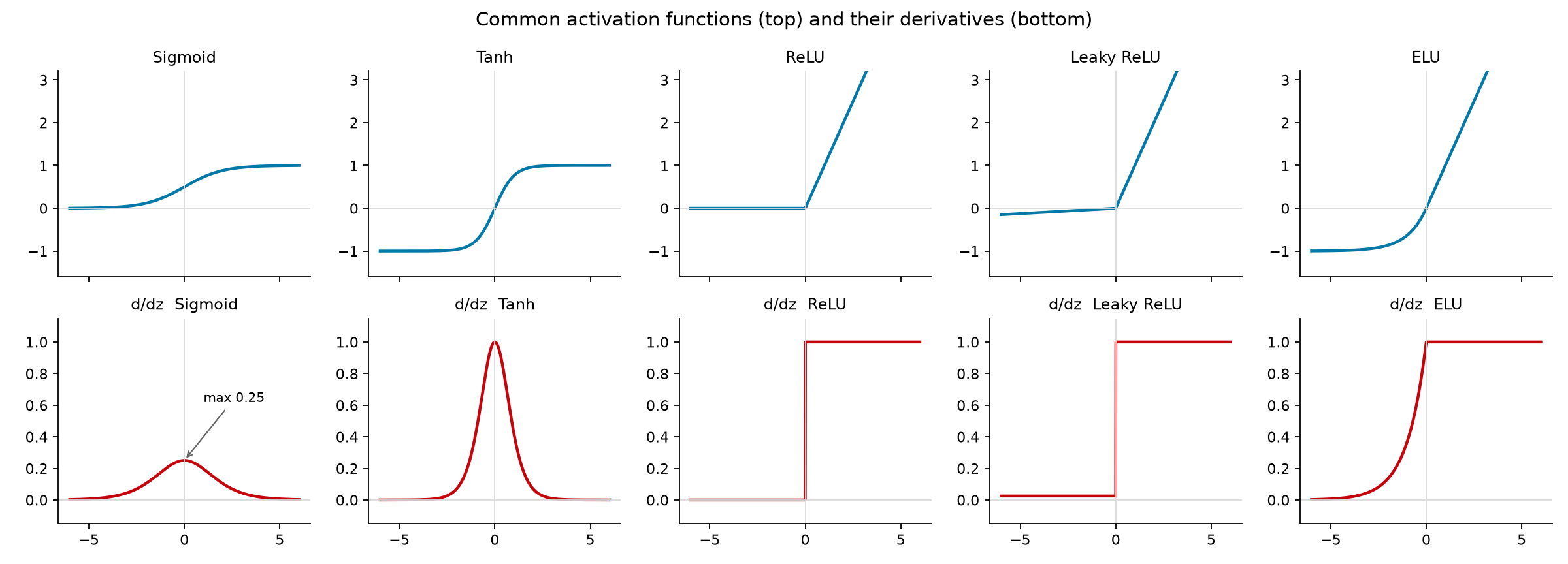
A Selection of Common Activations
The classical choices are the identity, the logistic sigmoid, tanh, and hard tanh:
The modern rectifier family replaces saturation on the positive side with a straight line:
Leaky ReLU fixes
Why Tanh Is Usually Preferred Over Sigmoid
Tanh has three advantages over the logistic sigmoid:
- Mean centering. Tanh is centered at zero, while the sigmoid outputs live in
(0, 1) and so carry a positive bias into the next layer.
- Positive and negative values. A unit can push the next layer in either direction.
- Larger gradients.
\tanh'(0) = 1 against\sigma'(0) = 0.25 , so the signal that survives a backward pass through a tanh layer is up to four times stronger.
Tanh also has a convenient derivative, expressible in terms of its own output:
These advantages only pay off if the unit actually operates near zero, where the derivative is largest. That is why it matters to normalize inputs to mean zero and to use random weight initialization centered at zero: both keep pre-activations in the high-gradient region instead of the flat tails.
The bottom row of the figure above also previews the gradient-flow problem that
Section 4 makes precise. Backpropagation multiplies one activation derivative per layer,
and
The Price: The Loss Is No Longer Convex
Every model in the course so far — linear regression, Adaline, logistic regression,
softmax regression — has a convex loss, so gradient descent converges to the global
minimum regardless of where it starts. Once nonlinear activations are inserted between
layers, that guarantee is gone: the deep loss is non-convex almost
always.
The practical consequence is a loss of reproducibility that surprises people the first
time they see it. Repeat the same training run, changing only the random seed for weight
initialization or the shuffling of the dataset, and you land in a different local
minimum with different final weights. Visualizations of deep loss surfaces show a
landscape of ridges, valleys and basins rather than a single
bowl.
This is less alarming than it sounds. As LeCun argued in “Who’s Afraid of Non-Convex
Loss Functions?”, convexity is overrated: choosing a suitable architecture matters more
than insisting on a convex objective, particularly when convexity restricts you to
architectures that cannot express the problem in the first place. Even for shallow
convex models such as SVMs, swapping in a non-convex loss can improve both accuracy and
speed.
Why We Initialize Randomly: Breaking Symmetry
A natural question at this point: what happens if we initialize an MLP to all-zero weights?
The answer is that the units stay symmetric forever. If every unit in a hidden layer
starts with identical weights, every unit computes the same pre-activation, receives the
same gradient in the backward pass, and therefore applies the same update. A layer of
This is exactly why we initialize randomly: random initialization breaks the symmetry so that different units can specialize on different features. Note the contrast with the perceptron of Lecture 4, where all-zero initialization was perfectly fine — a single unit has no siblings to be symmetric with. Combined with the requirement above that weights stay centered at zero, the constraints on initialization are becoming specific enough to deserve their own treatment, which is where principled schemes such as Xavier and He initialization come in later in the course.
Section 4: Backpropagation
Having introduced multilayer perceptrons and their activation functions, we now consider
how to learn their parameters. Training requires the gradient of the loss with respect to
every weight and bias. Backpropagation computes these gradients by applying the chain
rule backward through the network — the algorithm Rumelhart, Hinton and Williams
introduced for learning internal representations.
Notation and the Forward Pass
Consider a network with
We use column vectors throughout. If layer
During the forward pass we compute the prediction
Propagating the Loss Gradient Backward
Let
Using the forward equation, each downstream pre-activation is
Applying the chain rule and summing over every downstream unit the activation reaches,
This sum over downstream units is precisely a matrix-vector product. Applying the local activation derivative yields
Here
Gradients of Weights and Biases
Within a layer,
Collecting these entries gives an outer product:
Each weight gradient combines the signal arriving along that connection with the loss
sensitivity of the receiving unit. The resulting matrix has the same shape as
Starting at the Output Layer
Assume a binary classification task with a sigmoid output and binary cross-entropy:
Since
The same delta holds not only for sigmoid with BCE, but also for softmax with categorical cross-entropy, which is the closed form Section 1 arrived at from the categorical likelihood.
A Worked Example: Forward and Backward Passes on XOR
Consider the network
evaluated with binary cross-entropy. Its parameters and the selected training example are
The target is one because exactly one input bit is one. We carry extra decimal places to keep the intermediate values consistent.
Forward pass. The hidden pre-activations and activations are
Consequently,
Backward pass. At the output,
so the output-layer gradients are
Next, propagate through the output weights:
For ReLU the derivative is one at positive inputs and zero at negative inputs, so the
activation mask is
Finally,
There are two distinct reasons for zero weight gradients here. The second input is zero,
so all gradients in the second column of
Why Depth Makes Gradients Fragile
Because backpropagation relies on the chain rule, the gradient reaching the first layer depends on the product of the local derivatives of every layer that follows:
Each factor describes how one layer’s pre-activation changes with the preceding layer’s, including the effect of both the weights and the activation function. To reach an early layer, the gradient must pass through all of them.
This is where the problem arises. Repeated multiplication by small factors makes
gradients in early layers extremely small — the vanishing-gradient problem — and
repeated multiplication by large factors makes them very large — the
exploding-gradient problem. For intuition, a scalar factor of
The activation derivatives plotted in Section 3 explain part of this sensitivity:
| Activation | Derivative | Implication for gradient flow |
|---|---|---|
| Sigmoid | Can strongly attenuate gradients, especially in saturation. | |
| Tanh | Has derivative one at zero, but still saturates at large magnitudes. | |
| ReLU | One for |
Preserves the local gradient on its active branch and blocks it on its inactive branch. |
Activation derivatives are only part of the product, though: the weight matrices affect both its magnitude and its direction. ReLU therefore does not guarantee stable gradients, and tanh does not eliminate vanishing gradients. This motivates the later study of initialization and normalization.
Section 5: Practical Considerations for Training MLPs
Reading Training and Validation Curves
Checking the training and test loss or error is a simple and useful diagnosis. The curves carry a lot of information, especially about overfitting and underfitting. A validation plateau, or an error that starts increasing, is a sign of overfitting. Minibatch losses are noisy, so averaging or smoothing can reveal the underlying trend. The curves also say something about the learning rate: if it is too high, the error tends to oscillate.
One caveat worth knowing about is grokking: on some small algorithmic tasks, strong
generalization emerges long after the training data have been
fit.
Parameters versus Hyperparameters
Parameters are learned from training data through optimization; in the MLP considered here they are the entries of the weight matrices and bias vectors. Hyperparameters specify the model or the training procedure and are chosen by the practitioner.
| Learned parameters | Model and training choices |
|---|---|
| Weights and biases | Hidden-layer count and width; activation and loss functions |
| Learning rate, schedule, optimizer, minibatch size, and epoch budget | |
| Initialization, input normalization, random seed, and regularization settings |
Underfitting, Overfitting, and Model Capacity
A low training error is not always a positive signal. Limited capacity prevents a good fit to the training data; increasing capacity lowers training error, but excessive capacity may increase generalization error, which is usually estimated with test-set error. The result is a gap between fitting observed examples and predicting unseen ones: as training error falls, the model improves on data it has seen, but that improvement is not guaranteed to transfer.
A Practical Training Routine
Before a long run, check input values, label encoding, tensor shapes, and whether the output is compatible with the loss. Record the configuration and the seed, log loss and accuracy, and measure epoch times. If the loss behaves unexpectedly, inspect the setup before spending more computation. Change one hyperparameter at a time when diagnosing a problem, and repeat promising comparisons across runs.
The lecture summarizes each minibatch update as four steps:
- Clear previously accumulated parameter gradients (
zero_grad()). - Run the forward pass and compute the loss.
- Compute gradients with backpropagation (
backward()). - Apply the optimizer update (
step()).
Keeping these roles separate makes debugging easier: the forward pass determines the prediction, the backward pass computes sensitivities, and the optimizer changes the parameters.
Why Deep Instead of Merely Wide?
A classical universal approximation result states that a network with one hidden layer
and a suitable activation can approximate any continuous function on a compact domain
arbitrarily well, given sufficient width. Cybenko established such a result for
continuous sigmoidal activations
Depth offers a different route: expressing a function as a composition of simpler transformations. Connected layers reuse intermediate features, so the same expressiveness can be reached with fewer parameters, and earlier features become the inputs from which later ones are built. That composition also acts as a kind of regularization, since later layers are constrained by the behavior of earlier ones. This is one reason deep learning is concerned with representation learning rather than simply adding layers.
Architecture also introduces an inductive bias: assumptions that favor certain representations or solutions. A layered composition constrains how later features are built from earlier ones. Adding layers does not automatically reduce parameter count, computation time, or overfitting — those outcomes depend on layer widths, the target task, and the training procedure. Greater depth also lengthens the chain through which gradients must pass, creating exactly the optimization difficulties discussed above.
From Fully Connected Layers to CNNs
The next lecture introduces convolutional neural networks. The useful connection is that,
after arranging inputs and outputs as vectors, a convolutional layer is the same
equation as a fully-connected one,
The difference lies in the structure of
The chain rule is unchanged. The gradient with respect to the input of this linear
operation is still
Backpropagation therefore connects these architectures through one principle: propagate loss sensitivities backward through local operations, and add all contributions when a variable or parameter influences the loss through multiple paths.
Key Takeaways
- Matrix backpropagation collects the chain rule’s sums over downstream units into matrix-vector products.
- A weight gradient is the receiving unit’s error signal multiplied by the activation arriving along that connection.
- Gradient flow depends on both the activation derivatives and the weight matrices across successive layers.
- Training loss measures fit to observed examples; validation performance helps select capacity, hyperparameters, and stopping points.