Lecture 08: Convolutional Neural Networks

From image tasks and shared filters to convolution arithmetic, backpropagation, and PyTorch.

1. Today’s Roadmap

What CNNs can do
Why images are difficult for fully connected networks
Convolutional neural network basics
Cross-correlation versus convolution
CNNs and backpropagation
CNNs in PyTorch

Convolutional Neural Networks (CNNs) replace dense, position-specific connections with small filters that are reused across the input. The lecture emphasizes three main ideas: sparse connectivity, parameter sharing, and combining local patterns through many layers.

Recap from Lecture 7. Backpropagation applies the chain rule by summing contributions from every path through which a variable affects the loss. For a linear layer $z=Wa+b$, the input gradient is $\partial L/\partial a=W^\top\delta$, where $\delta=\partial L/\partial z$. Convolutional layers follow the same principle, with local connections and shared weights.

2. What CNNs Can Do

Image classification assigns a class or class probability to an entire image. The lecture shows a cat-versus-dog example where the network produces an output such as $p(y=\mathrm{cat})$.

Object detection identifies multiple objects and their locations in an image, usually by predicting bounding boxes around objects such as cars, people, and trucks.

Object segmentation predicts which pixels belong to objects or regions, so the model describes object shapes rather than only giving an image-level label or a bounding box.

3. Why Images Are Hard

The same object can appear differently under changes in lighting, contrast, viewpoint, or location. Even a simple translation moves the important pixels to different coordinates. This makes a purely position-specific representation inconvenient for image recognition.

A sufficiently wide fully connected network with suitable nonlinear activations can approximate continuous functions on a bounded, closed input domain. However, this does not tell us how many units or training examples are needed. CNNs introduce architectural assumptions about locality and repeated patterns that are particularly useful for images.

Full connectivity also creates a parameter problem. For a $3\times200\times200$ image, the first hidden-layer neuron would need 120,000 input weights, excluding its bias. A layer with many hidden neurons would multiply this count further. CNNs reduce this burden by connecting each output only to a small local region and by reusing the same weights in many locations. This reduces storage and can help generalization, although CNNs can still overfit.

4. Convolutional Neural Network Basics

A filter (or kernel) is a small set of weights that slides over the input. Instead of learning a different set of weights for every absolute pixel position, the same kernel is reused across many positions. This is parameter sharing.

The output of one filter is a feature map. The lecture describes a filter as a “feature detector”: a local detector that works in one region may also work when the same pattern appears elsewhere in the image.

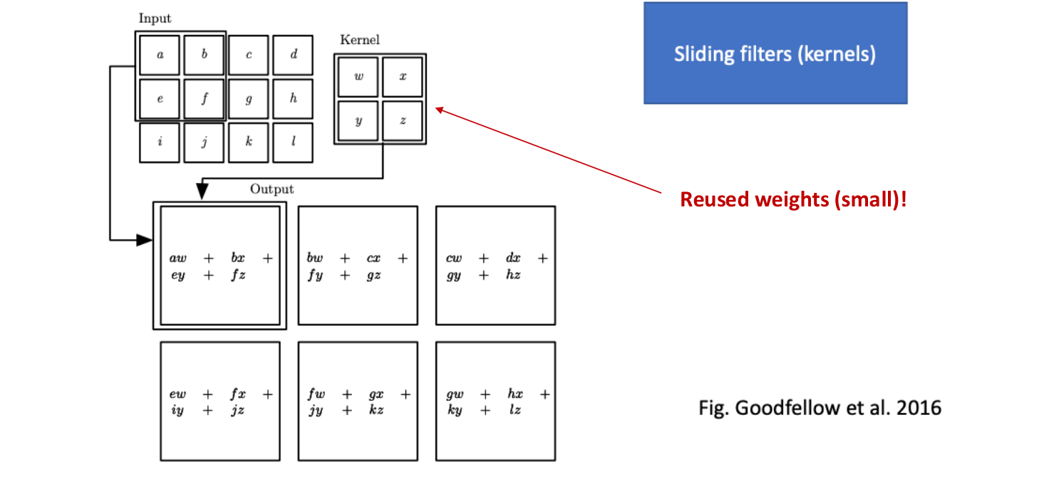
A 2 by 2 kernel slides across a 3 by 4 input to produce a 2 by 3 feature map. — **Figure 1. Weight sharing in a convolutional kernel.** The same small set of kernel weights is reused as the filter moves across the input. Reproduced from the lecture slides; the original source credit to Goodfellow et al. (2016) is retained in the image.

In Figure 1, the input has 3 rows and 4 columns, and the kernel has 2 rows and 2 columns. With stride 1 and no padding, the kernel fits in two vertical positions and three horizontal positions, producing a $2\times3$ feature map. Each output sums four input–weight products. The same four kernel weights are used at all six positions; bias is omitted in this illustration.

4.2 Input and Output Channels

CNNs normally learn multiple filters. Each filter produces its own feature map, so a hidden convolutional layer can be viewed as a collection of feature maps produced by different learned detectors.

An RGB image has three input channels. In a standard convolution, each filter contains a separate spatial slice of weights for each input channel. At each location, it sums the weighted values across all three channels, adds its bias, and produces one output value. One filter therefore produces one feature map, not three separate output maps.

For a $32\times32$ grayscale input, six $5\times5$ filters with stride 1 and no padding produce six $28\times28$ feature maps. This layer has one input channel and six output channels.

4.3 Pooling

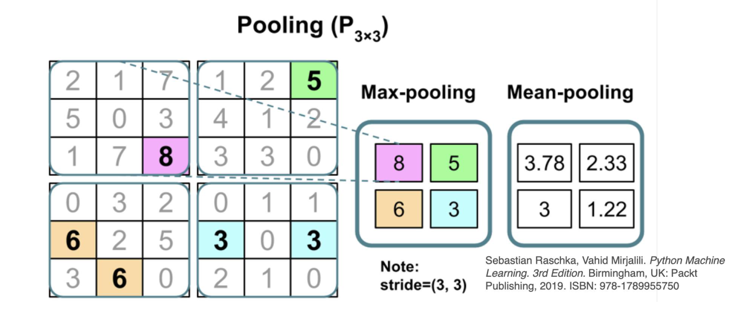
Pooling reduces the spatial size of a representation and is described in the lecture as lossy compression. In max-pooling, each region is replaced by its maximum value. In mean-pooling, each region is replaced by its average.

Max-pooling and mean-pooling summarize four 3 by 3 regions of a 6 by 6 input into 2 by 2 outputs. — **Figure 2. Max-pooling and mean-pooling.** Different pooling rules summarize a local region into a smaller output. Reproduced from the lecture slides; the original source credit to Raschka and Mirjalili (2019) is retained in the image.

The lecture summarizes the main ideas of CNNs as follows:

Sparse connectivity: one feature-map element connects only to a small patch of the input rather than to the entire image.
Parameter sharing: the same filter weights are reused for different spatial locations.
Many layers: local patterns extracted in early layers can be combined into larger and more global patterns in deeper layers.

Receptive field means the part of the original input that can affect a hidden activation. Although one convolutional unit initially sees only a local patch, receptive fields grow with depth because later units combine outputs from earlier local regions.

5. Cross-Correlation vs. Convolution

5.1 Convolution in Probability

Let $Z=X+Y$, where $X$ and $Y$ are independent. To obtain a particular sum $z$, every possible value $x$ must be paired with $z-x$. Independence lets us multiply the corresponding densities or probabilities, and we integrate or sum over all possible $x$.

For independent continuous random variables, with densities $f_X$ and $f_Y$,

f_Z(z)=\int_{-\infty}^{\infty} f_X(x)f_Y(z-x)\,dx.

For independent discrete random variables, the integral becomes a sum. Writing $p_X$, $p_Y$, and $p_Z$ for the probability mass functions,

p_Z(z)=\sum_x p_X(x)p_Y(z-x).

These operations are called convolutions. The continuous formula gives a density at $z$, not the probability of the single event $Z=z$.

5.2 The Operation Used in CNNs

A CNN forms an output by sliding a kernel over an activation window, multiplying aligned values, and summing them. The lecture points out an important terminology detail: what deep-learning frameworks usually call “convolution” is technically cross-correlation because the kernel is not flipped.

For a single input channel, omitting bias,

\text{Cross-correlation:}\qquad Z[i,j]=\sum_u\sum_v K[u,v]A[i+u,j+v].

\text{Convolution:}\qquad Z[i,j]=\sum_u\sum_v K[u,v]A[i-u,j-v].

Here, $A$ is the input activation map, $K$ is the kernel, and $u,v$ index kernel offsets. These expressions describe the operation before restricting it to the desired output positions and choosing a boundary convention.

True convolution flips the kernel horizontally and vertically relative to cross-correlation. In common deep-learning usage, however, the cross-correlation operation is still implemented by layers named convolution.

6. Output Size, Stride, and Padding

The spatial size of a convolution output depends on four quantities: input width $W$, kernel width $K$, padding $P$ on each side, and stride $S$. For the undilated convolution considered here, the lecture gives the output-width formula

O=\frac{W-K+2P}{S}+1.

Stride controls how far the kernel moves between neighboring positions. Padding adds values around the border of the input, allowing the kernel to operate near the boundary and changing the resulting output size.

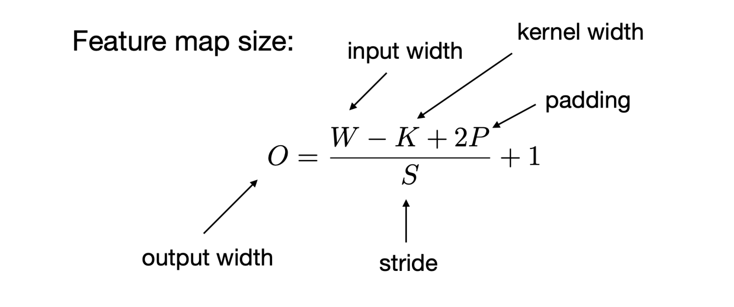
Output width equals input width minus kernel width plus twice the padding, divided by stride, plus one, when the division is exact. — **Figure 3. Convolution output size.** The output dimension depends on input width, kernel width, padding, and stride. Reproduced from the lecture slides. See also Dumoulin and Visin for convolution arithmetic.

This expression assumes that $(W-K+2P)$ is an integer multiple of $S$; otherwise, round the quotient down before adding 1. Apply the formula separately to height and width.

For a $28\times28$ grayscale input, eight $5\times5$ filters with stride 1 and no padding give $O=(28-5)/1+1=24$. The output shape is $8\times24\times24$, written as channels × height × width and excluding the batch dimension.

The lecture also cautions that CNNs are not automatically invariant to translation, rotation, or scale. Weight sharing lets the same detector be applied at different locations, but the resulting activations can still depend on where and how an object appears.

Data augmentation trains the model on label-preserving transformations, such as suitable shifts or crops, so it can learn to give consistent predictions across those variations. This encourages robustness but does not guarantee perfect invariance.

7. CNNs and Backpropagation

Backpropagation in CNNs uses the same multivariable chain rule as before, with one additional constraint: weights are shared. Because one kernel weight is reused in multiple positions, the gradient for that weight must collect contributions from every computational path in which the shared weight appears.

7.1 Backpropagation Through a 1D Convolution

For a 1D cross-correlation with a kernel of size 2, the lecture defines input activations $a=(a_1,a_2,a_3,a_4)$ and a shared kernel $(w_1,w_2)$. With stride 1, no padding, and no bias, the 1D cross-correlation produces

z_k=w_1a_k+w_2a_{k+1},\qquad k=1,2,3.

Define the incoming gradient from the rest of the network as

\delta_k=\frac{\partial L}{\partial z_k}.

It measures how sensitive the final loss is to $z_k$. We use it to compute gradients for this layer’s inputs and weights.

Input $a_2$ appears in $z_1$ with coefficient $w_2$ and in $z_2$ with coefficient $w_1$. The chain rule therefore gives

\frac{\partial L}{\partial a_2} =\frac{\partial L}{\partial z_1}\frac{\partial z_1}{\partial a_2} +\frac{\partial L}{\partial z_2}\frac{\partial z_2}{\partial a_2} =\delta_1w_2+\delta_2w_1.

Applying the same reasoning to all four inputs,

\frac{\partial L}{\partial a_1}=w_1\delta_1,

\frac{\partial L}{\partial a_2}=w_2\delta_1+w_1\delta_2,

\frac{\partial L}{\partial a_3}=w_2\delta_2+w_1\delta_3,

\frac{\partial L}{\partial a_4}=w_2\delta_3.

Each kernel weight is used at all three output positions, so its gradient sums contributions from all three uses:

\frac{\partial L}{\partial w_1}=\delta_1a_1+\delta_2a_2+\delta_3a_3,

\frac{\partial L}{\partial w_2}=\delta_1a_2+\delta_2a_3+\delta_3a_4.

The optimizer uses these weight gradients to update the kernel. Weight sharing changes which contributions must be added; it does not change the chain rule.

7.2 Numerical Example

Using $w=(2,-1)$ and $\delta=(1,3,-2)$, the lecture obtains

\frac{\partial L}{\partial a}=(2,5,-7,2).

The same result can be viewed as zero-padding $\delta$ to $(0,1,3,-2,0)$ and cross-correlating it with the flipped kernel $(-1,2)$. This connects the backward calculation to another convolution-like operation rather than treating it as a completely different procedure.

8. CNNs in PyTorch

The lecture shows a LeNet-style network in PyTorch. Its feature extractor alternates convolution, nonlinear activation, and max-pooling; the resulting feature maps are then flattened and passed to fully connected layers for classification.

The following is an architecture sketch, not a complete executable program:

nn.Conv2d(in_channels, 6, kernel_size=5)
nn.Tanh()
nn.MaxPool2d(kernel_size=2)
nn.Conv2d(6, 16, kernel_size=5)
nn.Tanh()
nn.MaxPool2d(kernel_size=2)
torch.flatten(x, 1)
nn.Linear(...), nn.Tanh(), nn.Linear(...)

The key idea is structural: convolution and pooling perform the spatial feature extraction, while the final fully connected layers use those learned features to produce class outputs.

9. Convolutions Beyond Images

The lecture closes by asking whether convolution-like ideas can be used for non-image data and briefly introduces Graph Convolutional Networks. Images have a regular grid structure, but other datasets have irregular connections, such as cities connected by roads. This extends the general idea of exploiting local structure and shared operations to graph-structured inputs.

10. Summary

CNNs can be used for image classification, object detection, and object segmentation.
Fully connected image models can require very large numbers of parameters.
A convolutional filter is a small set of weights reused across spatial locations.
Sparse connectivity and parameter sharing are central structural ideas in CNNs.
Multiple filters produce multiple feature maps, and receptive fields grow through depth.
Pooling reduces spatial resolution using summaries such as a maximum or mean.
Deep-learning “convolution” layers usually compute cross-correlation rather than a mathematically flipped convolution.
Output size depends on input size, kernel size, padding, and stride.
CNN backpropagation still uses the chain rule, while accounting for shared weights and multiple gradient paths.
PyTorch combines convolution, activation, pooling, flattening, and fully connected layers to build CNNs.
CNNs still require architectural choices and can overfit; weight sharing alone does not guarantee invariance.

Lecture Source

Lengerich, B. STAT 453 Lecture 08 slides, September 29, 2026.