Lecture 10: Normalization / Initialization

Input normalization, batch normalization, and weight initialization.

1. Input Normalization

Normalization and Gradient Descent

Problem: When input features have very different scales, the cost function may have elongated elliptical contours, causing gradient descent to zigzag toward the minimum.
Why: Gradient descent uses the same learning rate for all weights. Differences in feature scales can cause some weights to receive much larger updates than others.
Goal: Scale input features so that weights such as $w_1$ and $w_2$ have more balanced effects on optimization, allowing gradient descent to approach the minimum more directly.

Standardization of Input Features

x_j^{[i]} = \frac{x_j^{[i]}-\mu_j}{\sigma_j}

Scaled features will have zero mean and unit variance.

In Deep Models…

Normalizing the inputs only affects the first hidden layer… what about the rest?

2. Batch Normalization

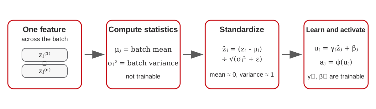
Input normalization gives the first hidden layer well-scaled data, but it does not directly control the values produced inside a deep network. Batch normalization (BatchNorm) applies the same basic idea to a hidden layer: for each hidden unit (or feature), it uses the current mini-batch to standardize that unit’s pre-activations, then learns a scale and shift. Keeping intermediate values on a controlled scale can make deep networks easier and more stable to optimize; Section 4 examines the competing explanations for why this works.

The word batch matters. BatchNorm compares one feature across examples in the mini-batch. It does not combine different features of one example. Later sections contrast this with LayerNorm, which normalizes within each example.

What Exactly Is Being Normalized?

Suppose a mini-batch contains $n$ examples. Let $z_j^{[i]}$ be the net input, or pre-activation, of hidden unit $j$ for example $i$. For instance, in a fully connected layer,

z^{[i]} = W a^{[i]} + b.

Fix one unit $j$. BatchNorm looks at the $n$ numbers $z_j^{[1]},\ldots,z_j^{[n]}$. Every hidden unit is normalized separately, so unit $j$ has its own statistics and its own learned parameters.

Four-stage BatchNorm pipeline: collect one feature across a mini-batch, compute its mean and variance, normalize it, then apply learned scale and shift before the activation. — **The BatchNorm pipeline for one hidden feature.** The same two-step transformation is applied independently to every feature. The mini-batch supplies the statistics; gradient descent learns the scale and shift.

Step 1: Standardize with Mini-Batch Statistics

First compute the mini-batch mean and variance for feature $j$:

\mu_j = \frac{1}{n}\sum_{i=1}^{n}z_j^{[i]}, \qquad \sigma_j^2 = \frac{1}{n}\sum_{i=1}^{n}\left(z_j^{[i]}-\mu_j\right)^2.

Then standardize each example:

\widehat{z}_j^{[i]} = \frac{z_j^{[i]}-\mu_j}{\sqrt{\sigma_j^2+\epsilon}}.

The small constant $\epsilon$ (often around $10^{-5}$) prevents division by zero and improves numerical stability. Within the current mini-batch, the normalized values have mean approximately zero and variance approximately one. The variance here uses $1/n$: BatchNorm is describing this batch, not constructing an unbiased population estimator.

Step 2: Learn the Useful Scale and Location

Forcing every hidden feature to remain at exactly zero mean and unit variance would be too restrictive. BatchNorm therefore follows standardization with a learned affine transformation:

u_j^{[i]} = \gamma_j\widehat{z}_j^{[i]} + \beta_j, \qquad a_j^{[i]} = \phi\!\left(u_j^{[i]}\right).

$\gamma_j$ controls the feature’s scale or spread.
$\beta_j$ controls the feature’s location or mean.
Both are trainable parameters, shared across all examples but different for each feature.

This second step means BatchNorm can learn more than plain standardization. If the network needs a different scale or offset, $\gamma_j$ and $\beta_j$ can restore it. In particular, $\beta_j$ usually makes the bias in the preceding linear layer redundant: adding the same bias to every example is canceled when the batch mean is subtracted. That is why a common pattern is Linear(..., bias=False) -> BatchNorm -> activation.

A Small Numerical Example

Suppose one hidden unit produces the three pre-activations $[1,2,3]$. Ignoring the tiny $\epsilon$ for readability,

\mu = 2, \qquad \sigma^2 = \frac{2}{3}, \qquad \widehat{z} \approx [-1.225,\ 0,\ 1.225].

If the layer learns $\gamma=0.5$ and $\beta=1$, its output before the activation is

u = 0.5\widehat{z}+1 \approx [0.388,\ 1,\ 1.612].

The example separates the two jobs clearly: the batch statistics standardize the three values, while the learned parameters choose the scale and center that the network finds useful.

BatchNorm Is Differentiable

The batch mean, variance, standardization, scale, and shift are all differentiable, so the whole layer can be trained with backpropagation. If $g_j^{[i]}=\partial L/\partial u_j^{[i]}$ is the gradient arriving from the next operation, the learned parameters have especially simple gradients:

\frac{\partial L}{\partial \beta_j} = \sum_{i=1}^{n} g_j^{[i]}, \qquad \frac{\partial L}{\partial \gamma_j} = \sum_{i=1}^{n} g_j^{[i]}\widehat{z}_j^{[i]}.

The gradient with respect to an input $z_j^{[i]}$ has more paths. That value affects its own normalized output directly, but it also changes $\mu_j$ and $\sigma_j^2$, which are used to normalize every example in the batch. The multivariable chain rule therefore has the structure

\frac{\partial L}{\partial z_j^{[i]}} = \frac{\partial L}{\partial \widehat{z}_j^{[i]}} \frac{1}{\sqrt{\sigma_j^2+\epsilon}} + \frac{\partial L}{\partial \mu_j}\frac{1}{n} + \frac{\partial L}{\partial \sigma_j^2} \frac{2\left(z_j^{[i]}-\mu_j\right)}{n}.

The main intuition is more important than memorizing this expression: examples in the same mini-batch become coupled through their shared mean and variance. Autograd keeps track of these paths automatically.

What to Remember

BatchNorm normalizes one hidden feature across the examples in a mini-batch.
Standardization uses the batch mean, batch variance, and a small $\epsilon$.
The learned $\gamma$ and $\beta$ parameters restore whatever scale and offset are useful.
Because the statistics depend on the whole batch, one example can affect the normalized values and gradients of the others.

The next section turns this mathematical layer into PyTorch code. Later sections explain what changes at test time and why BatchNorm can help optimization.

3. BatchNorm in PyTorch

BatchNorm in PyTorch

class MultilayerPerceptron(torch.nn.Module):

    def __init__(self, num_features, num_classes, drop_proba,
                 num_hidden_1, num_hidden_2):
        super().__init__()

        self.my_network = torch.nn.Sequential(
            # 1st hidden layer
            torch.nn.Flatten(),
            torch.nn.Linear(num_features, num_hidden_1, bias=False),
            torch.nn.BatchNorm1d(num_hidden_1),
            torch.nn.ReLU(),

            # 2nd hidden layer
            torch.nn.Linear(num_hidden_1, num_hidden_2, bias=False),
            torch.nn.BatchNorm1d(num_hidden_2),
            torch.nn.ReLU(),

            # output layer
            torch.nn.Linear(num_hidden_2, num_classes)
        )

    def forward(self, x):
        logits = self.my_network(x)
        return logits

Source: https://github.com/rasbt/stat453-deep-learningss21/blob/main/L11/code/batchnorm.ipynb

Training and Testing

Don’t forget model.train() and model.eval() in training and test loops.

BatchNorm at Test-Time

Use exponentially weighted average (moving average) of mean and variance.

running_mean = momentum * running_mean + (1 - momentum) * sample_mean

Where momentum is typically ~0.1; same for variance.
Alternatively, can also use global training set mean and variance.

4. Why Does BatchNorm Work?

Batch normalization can improve training speed and stability. However, researchers have proposed several explanations for its effectiveness.

Internal Covariate Shift

Ioffe and Szegedy (2015) originally introduced BatchNorm to reduce internal covariate shift. During training, updates to earlier layers change the distribution of inputs received by later layers. Normalizing these inputs was intended to reduce these distributional changes and make training easier.

Later research questioned whether reducing internal covariate shift is the main reason BatchNorm works.

Smoother Optimization and Larger Learning Rates

Santurkar et al. (2018) argued that BatchNorm makes the optimization landscape smoother. This produces more predictable and stable gradients, allowing faster training and larger learning rates.

The lecture presents two experiments supporting this interpretation:

A VGG network trained on CIFAR-10 with BatchNorm trained faster and tolerated a larger learning rate than the network without BatchNorm.
Adding time-varying noise to BatchNorm outputs made their distributions less stable, but the model still trained nearly as well as the standard BatchNorm model.

These results suggest that stable layer input distributions are not necessary for BatchNorm’s training benefits.

Other Interpretations and Limitations

The lecture discusses several additional findings:

Reduced reliance on individual directions: Morcos et al. (2018) found that BatchNorm implicitly discourages reliance on individual units or particular linear combinations of units.
Implicit regularization: Luo et al. (2018) studied how BatchNorm can act as a regularizer and improve generalization.
Potential gradient instability: Yang et al. (2019) showed that BatchNorm can cause exploding gradients in deep networks without skip connections. Careful tuning may therefore still be necessary.

BatchNorm’s effectiveness should not be attributed solely to reducing internal covariate shift.

Practical Considerations

BatchNorm estimates the mean and variance from each mini-batch. Larger batches generally provide more stable estimates. With very small batches, such as four or fewer examples, these estimates can become noisy. This is relevant during fine-tuning or when memory constraints limit the batch size.

Two common approaches are:

Freeze BatchNorm: Use stored running statistics instead of recomputing statistics from the current small batch.
Use GroupNorm: Normalize groups of channels within each example, avoiding dependence on batch size.

GroupNorm connects related normalization methods: one group corresponds to LayerNorm over the same dimensions, while one channel per group corresponds to InstanceNorm.

Unlike BatchNorm, which computes statistics across examples in a mini-batch, LayerNorm computes statistics across features within an example. LayerNorm is commonly used in Transformers.

The lecture also raises the question of whether BatchNorm should be placed before or after the activation function. This is a design consideration when choosing a network architecture.

5. Weight Initialization: Why Do We Care?

Weight initialization determines the starting values of a neural network’s parameters. Two important considerations are breaking symmetry between neurons and choosing an appropriate weight scale.

6. Xavier & He Initialization

Proper weight initialization helps maintain stable activations and gradients as information passes through multiple layers of a neural network. Two commonly used initialization methods are Xavier initialization and He initialization.

6.1 Xavier Initialization

Xavier initialization, also known as Glorot initialization, was introduced by Glorot and Bengio (2010). Its main goal is to keep the variance of activations during the forward pass and gradients during the backward pass approximately stable across layers.

The method consists of two steps:

Initialize the weights randomly using a Gaussian or uniform distribution.
Scale the weights according to both the number of inputs (fan-in) and outputs (fan-out) of the layer.

For Xavier initialization, the weight variance is:

\operatorname{Var}(W) = \frac{2}{n_{\text{in}} + n_{\text{out}}}

Here:

fan-in ($n_{\mathrm{in}}$): Number of input connections to the layer.
fan-out ($n_{\mathrm{out}}$): Number of output connections from the layer.
Var(W): Variance of the initialized weights.

By accounting for both input and output dimensions, Xavier initialization aims to prevent activation and gradient magnitudes from becoming excessively large or small as they propagate through a deep neural network.

6.2 Derivation of the Forward-Pass Variance

To understand why the initialization scale depends on the number of inputs, consider the pre-activation of neuron $j$ in layer $l$:

z_j^{(l)} = \sum_{k=1}^{m^{(l-1)}} W_{jk}^{(l)} \, a_k^{(l-1)}

where:

$W_{jk}^{(l)}$ is the weight connecting neuron $k$ in the previous layer to neuron $j$ in the current layer.
$a_k^{(l-1)}$ is the activation of neuron $k$ in the previous layer.
$m^{(l-1)}$ is the number of neurons in the previous layer, corresponding to fan-in.

Assuming independent terms, zero-mean weights and activations, and common weight and activation variances across their respective indices, we obtain:

\operatorname{Var}\left(z_j^{(l)}\right) = m^{(l-1)} \cdot \operatorname{Var}\left(W^{(l)}\right) \cdot \operatorname{Var}\left(a^{(l-1)}\right)

This shows that the variance of the pre-activation increases with the number of inputs if the weight variance remains constant.

To preserve approximately the same variance during the forward pass, we therefore want:

\operatorname{Var}\left(W^{(l)}\right) \approx \frac{1}{m^{(l-1)}}

This simplified derivation considers only forward propagation, so it depends on fan-in alone. When backward propagation is also considered, fan-out becomes important, leading to the full Xavier initialization formula introduced above.

6.3 He Initialization

He initialization, also called Kaiming initialization, was introduced by He et al. (2015). It is designed particularly for neural networks that use the ReLU activation function.

Xavier initialization relies on assumptions that are more suitable for activations such as tanh. However, ReLU behaves differently:

\mathrm{ReLU}(x)=\max(0,x)

ReLU sets negative inputs to zero. When the inputs are approximately symmetrically distributed around zero, roughly half of them are set to zero.

To account for this behavior, He initialization uses a larger weight variance:

\mathrm{Var}(W)=\frac{2}{n_{\mathrm{in}}}

Equivalently, starting from random weights with unit variance, the weights can be scaled by:

W^{(l)}\leftarrow W^{(l)} \sqrt{\frac{2}{m^{(l-1)}}}

Compared with the forward-only scaling derived earlier, He initialization introduces an additional factor of $\sqrt{2}$ to compensate for the effect of ReLU.

The main distinction: Xavier initialization considers both fan-in and fan-out to balance signal propagation, while He initialization uses a ReLU-specific scaling primarily based on fan-in.

6.4 Initialization Beyond Xavier and He

The appropriate initialization strategy depends on the neural network architecture. As neural network models evolve, initialization methods may also need to change.

For example, Transformer architectures may require different initialization considerations. Research on extremely deep neural networks also studies the spectrum of weight matrices and uses ideas from random matrix theory to develop initialization methods for networks with thousands of layers.

7. Weight Initialization Schemes in PyTorch

PyTorch provides built-in initialization methods that automatically initialize neural network parameters.

7.1 Default Weight Initialization in PyTorch

When a torch.nn.Linear layer is created, PyTorch initializes its weights and biases through the reset_parameters() method.

The implementation shown in the lecture is:

def reset_parameters(self):
    init.kaiming_uniform_(self.weight, a=math.sqrt(5))
    if self.bias is not None:
        fan_in, _ = init._calculate_fan_in_and_fan_out(self.weight)
        bound = 1 / math.sqrt(fan_in) if fan_in > 0 else 0
        init.uniform_(self.bias, -bound, bound)

The initialization process includes:

Weights: kaiming_uniform_() initializes the weight matrix.
Fan-in: PyTorch calculates the number of input connections.
Biases: Bias values are sampled from a uniform distribution based on fan-in.

Note that a=math.sqrt(5) makes PyTorch’s default initialization different from the standard ReLU-specific He initialization discussed in Section 6.3.

7.2 Key Takeaway

Xavier and He initialization help maintain stable signal propagation across network layers. PyTorch provides built-in methods to initialize weights automatically, making deep neural networks easier to train.

Breaking Symmetry

Initializing all weights to zero creates a symmetry problem. Neurons in the same hidden layer begin with identical parameters, produce identical outputs, and receive identical updates. They therefore fail to learn different features.

Random initialization breaks this symmetry by giving neurons different starting weights.

Choosing the Weight Scale

The lecture emphasizes starting with relatively small weights. Traditional initialization methods include:

Sampling from a uniform distribution, such as [0, 1], or preferably a distribution centered around zero, such as [-0.5, 0.5].
Sampling from a Gaussian distribution with mean zero and a small variance, such as 0.1 or 0.01.