Generative versus discriminative models through logistic regression and Naive Bayes, then autoencoders and their variants as a first step toward deep generative models.
1. Generative and Discriminative Models
Notation. Throughout these notes, uppercase X and Y denote random variables for an observed input (such as an image or a feature vector) and its class label (such as “cat” or “dog”). Lowercase x and y denote particular values of them. Following the slides, the training examples in Section 2 are written (X_i, Y_i), with i indexing examples. When a distribution depends on model parameters \theta, we write them after a semicolon, as in P(Y \mid X; \theta). For a continuous input, P(X \mid Y) should be read as a density.
1.1 From Classification to Generative Modeling
Much of the deep learning material covered earlier in the course focused on discriminative models: models that take an observation as input and make a prediction. For example, an image classifier takes an image of an animal and predicts whether it is a cat or a dog. The central question is “Given this input, what is its label?”
Deep generative models, the focus of the second half of the course, offer a different perspective. Instead of learning only how to label an observed example, they aim to learn the probability structure of the data itself. Such a model can be used to produce new examples that resemble its training data, which is what modern generative AI systems such as chatbots and image generators do. Generative AI has become a major technological and economic force, which is part of the motivation for studying these models.
A useful distinction is that classification asks which class an existing observation belongs to, whereas generation concerns how observations arise and how new observations can be sampled. A generative model can nevertheless be used for classification, as explained below.
1.2 What Distribution Does Each Approach Model?
A discriminative model directly learns the conditional distribution of the label given the input:
P(Y\mid X).
For example, P(Y=\mathrm{cat}\mid X=x) is the probability that a particular image x depicts a cat. This approach focuses on predicting Y after X is observed; it does not require a model for the overall distribution of images P(X).
A generative model, in the supervised setting of this lecture, models the joint distribution:
P(X,Y).
The joint distribution characterizes how inputs and labels occur together. By the product rule of probability, it can be factorized as
P(X,Y)=P(X\mid Y)P(Y).
Here, P(Y) is the prior class probability, and P(X\mid Y) describes the distribution of observations within a given class. Learning these quantities provides a route to the conditional probability needed for classification.
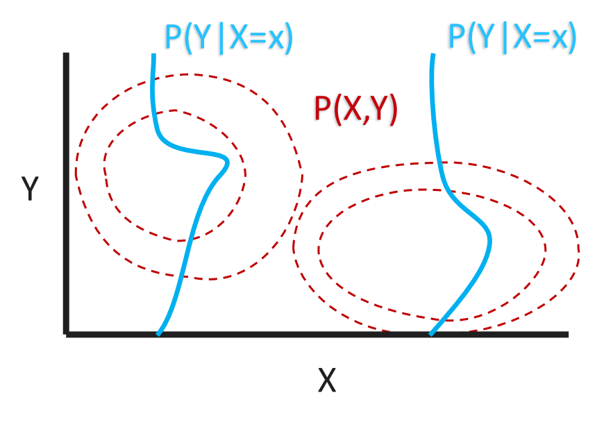
Figure 1. Joint versus conditional distributions.
The dashed contour lines show the joint density P(X,Y), which here has two clusters. Each solid curve is a conditional distribution P(Y\mid X=x): a vertical slice through the joint density at one fixed input value x. A generative model describes the whole joint density, whereas a discriminative model only describes the slices. Figure from the lecture slides.
1.3 Two Paths to the Same Posterior Probability
Suppose the training data contain observed input–label pairs (X, Y). Both approaches can produce a posterior probability P(Y\mid X), but they obtain it in different ways.
Discriminative route: Learn P(Y\mid X) directly from labeled observations. No explicit model of P(X) is required.
Generative route: Learn the class-conditional distribution P(X\mid Y) and the class prior P(Y), then apply Bayes’ theorem:
P(Y\mid X)=\frac{P(X\mid Y)P(Y)}{P(X)}.
In this expression:
P(Y\mid X)
is the posterior probability of the label after observing the input.
P(X\mid Y)
is the likelihood of the input under the class.
P(Y)
is the prior probability of that class.
P(X)
is the marginal probability (or evidence) of the observed input, which normalizes the posterior probabilities.
For a discrete set of possible labels \mathcal{Y}, the denominator is obtained by summing the joint distribution over the labels:
P(X)=\sum_{y\in\mathcal{Y}}P(X\mid Y=y)P(Y=y).
The lecture writes this marginalization in its general form as an integral, P(X)=\int_Y P(X,Y)\,dY, which is what one would use if Y were continuous. For a classification problem such as cat versus dog, Y is discrete and the integral becomes the sum above. In either case, the denominator ensures that the resulting posterior distribution is properly normalized.
1.4 Two Paths to Classification
Once a model can evaluate class probabilities, it can select a predicted label \hat{Y}. Here, argmax means the label that makes the given expression largest.
For a discriminative model, the classification rule is
For a fixed observed input x, the denominator P(X=x) is the same for every candidate class y. Therefore, it does not affect which class has the highest score, and the rule simplifies to
This is why, in the lecture, the step “calculate P(X)” is crossed out on the generative path to classification. It explains an important distinction between computing a normalized posterior and choosing the most likely class: calculating P(Y\mid X) requires the normalization term, but identifying the class with the greatest posterior probability does not.
Illustrative example (added to clarify the lecture): Suppose an image x has class-conditional scores P(x\mid \mathrm{cat})=0.6 and P(x\mid \mathrm{dog})=0.3, with prior probabilities P(\mathrm{cat})=0.4 and P(\mathrm{dog})=0.6. The unnormalized posterior scores are
Since 0.24>0.18, the generative classifier predicts cat. If normalized class probabilities are needed, the scores sum to 0.42, giving P(\mathrm{cat}\mid x)=0.24/0.42\approx0.571 and P(\mathrm{dog}\mid x)=0.18/0.42\approx0.429. These numbers are an explanatory example, not values from the lecture; for a continuous input they can be interpreted as probability densities.
1.5 Key Takeaways
Discriminative models directly learn P(Y\mid X), making them natural tools for predicting labels.
Generative models describe P(X,Y), often through P(X\mid Y)P(Y), and can obtain class probabilities using Bayes’ theorem.
Both approaches can perform classification, but their learning objectives and the distributions they explicitly represent differ.
When predicting the most probable class with a generative model, the common normalization factor P(X) can be omitted inside the \mathop{\mathrm{argmax}}.
2. Logistic Regression vs. Naive Bayes
Section 1 described two routes to the posterior P(Y \mid X). This section makes each route concrete with a classic example: logistic regression for the discriminative route and Gaussian Naive Bayes for the generative route. For simplicity we use a binary label Y \in \lbrace 0, 1 \rbrace and a feature vector X = (X_1, \ldots, X_d)^T \in \mathbb{R}^d. The training set consists of pairs (X_i, Y_i) for i = 1, \ldots, n, where the subscript i indexes training examples and the subscript j (used below) indexes features.
2.1 A Discriminative Model: Logistic Regression
Logistic regression follows the discriminative route: observe (X, Y) and learn P(Y \mid X) directly.
where \theta \in \mathbb{R}^d is the weight vector, \theta^T X = \sum_{j=1}^{d} \theta_j X_j is a linear score, and
\sigma(z) = \frac{1}{1 + e^{-z}}
is the sigmoid (logistic) function. The sigmoid maps any real number z to the interval (0, 1), so its output can be read as a probability. A bias (intercept) term is included by treating one of the d features as the constant X_0 = 1, so it does not need separate notation.
Why this parameterization? The sigmoid is not an arbitrary choice. Take the log-odds of the positive class, i.e., the log of the ratio between the probabilities of the two classes. Writing s = \theta^T X,
So logistic regression is exactly the model in which the log-odds are a linear function of the features. Each weight \theta_j is the change in the log-odds when feature X_j increases by one unit with the other features held fixed. The decision boundary P(Y=1 \mid X) = 0.5 is the hyperplane \theta^T X = 0, so logistic regression is a linear classifier.
2.2 Estimating Logistic Regression
Maximum likelihood. The parameters are fit by maximizing the conditional likelihood of the observed labels given the observed features. Assuming the training examples are independent,
Because Y_i is 0 or 1, the two cases of the model can be written as one Bernoulli expression, P(Y_i \mid X_i; \theta) = \sigma(\theta^T X_i)^{Y_i} \, \big(1 - \sigma(\theta^T X_i)\big)^{1 - Y_i}. Taking the logarithm (which is increasing, so it does not change the argmax) turns the product into a sum:
The bracketed term is the negative of the binary cross-entropy loss, so maximizing this log-likelihood is the same as minimizing the cross-entropy loss used to train classifiers earlier in the course.
There is no closed-form solution for \hat{\theta}. The log-likelihood is concave in \theta, though, so gradient-based methods find the global optimum. Its gradient has a simple form (a standard result, added here for completeness):
where \ell(\theta) is the log-likelihood above. Each example pushes \theta in the direction of its features, scaled by its prediction error Y_i - \sigma(\theta^T X_i).
Prediction. For a new input X, compute P(Y=1 \mid X) = \sigma(\hat{\theta}^T X) directly. No model of X itself and no Bayes’ theorem are involved.
2.3 A Generative Model: Naive Bayes
Naive Bayes follows the generative route: learn the class-conditional distribution P(X \mid Y) and the class prior P(Y), then obtain the posterior with Bayes’ theorem,
P(Y \mid X) = \frac{P(X \mid Y) \, P(Y)}{P(X)}.
The “naive” assumption. Modeling P(X \mid Y) for a d-dimensional X is hard in general, because the features can depend on each other in complicated ways. Naive Bayes assumes the features are conditionally independent given the class:
P(X \mid Y) = \prod_{j=1}^{d} P(X_j \mid Y).
As a graphical model, the label Y is the single parent of every feature node X_1, \ldots, X_d, with no edges between features (Y \to X_1, \; \ldots, \; Y \to X_d). Once the class is known, learning the value of one feature tells us nothing more about any other feature. This is rarely exactly true (for example, neighboring pixels in an image are strongly correlated even within one class), but it reduces one d-dimensional estimation problem to d one-dimensional ones.
Class-conditional distributions. For continuous features, the lecture uses a Gaussian for each feature in each class (Gaussian Naive Bayes):
where \mu_{jk} and \sigma_{jk}^2 are the mean and variance of feature j among examples of class k. (Here \sigma_{jk} is a standard deviation, not the sigmoid function of Section 2.1.)
Class prior. The prior is the frequency of each label in the training data:
P(Y = k) = \frac{\#\lbrace\text{samples with } Y = k\rbrace}{\text{total number of samples}} = \frac{n_k}{n}.
2.4 Estimating Naive Bayes
Maximum likelihood. The lecture writes the estimation step as
i.e., choose the Gaussian parameters that make the observed features most probable given their observed labels. Section 3.2 instead writes the Naive Bayes estimate as maximizing the joint likelihood P(X, Y; \theta). The two agree: since P(X, Y) = P(X \mid Y) P(Y), and the Gaussian parameters appear only in P(X \mid Y) while the class probabilities appear only in P(Y), maximizing the joint likelihood splits into this fit and the prior estimate n_k / n from Section 2.3. Because of the factorization, the Gaussian fit itself further decomposes into a separate one-dimensional Gaussian fit for every pair (feature j, class k), and each fit has a closed-form solution, the sample mean and sample variance within that class:
where X_{ij} is the value of feature j in example i and n_k is the number of examples in class k. The prior estimate n_k / n from Section 2.3 is likewise the maximum likelihood estimate of a categorical distribution. Training is therefore a single pass over the data with no iterative optimization, in contrast to logistic regression.
Prediction. Plug the estimates into Bayes’ theorem:
As noted in Section 1.4, the denominator P(X) is needed only to report a normalized probability. To choose the most likely class, it is enough to compare the numerators \prod_j P(X_j \mid Y = k) P(Y = k) across classes.
2.5 How the Two Models Relate
Both models end up producing P(Y \mid X), but they get there differently: logistic regression maximizes the conditional likelihood iteratively, while Naive Bayes fits class-conditional Gaussians and label frequencies in closed form and then applies Bayes’ theorem. Section 3.2 gives the lecture’s side-by-side comparison.
The two models are also more closely related than this description suggests. If the Gaussian Naive Bayes variances are shared across classes (\sigma_{j0} = \sigma_{j1} = \sigma_j), then the log-odds \log \frac{P(Y=1 \mid X)}{P(Y=0 \mid X)} implied by Naive Bayes is a linear function of X, so its posterior has exactly the logistic-regression form \sigma(\beta^T X) for some weight vector \beta determined by the means, variances and priors. (This result was not covered in lecture; it is added because it explains why the two are a natural pair, and it is the reason Ng and Jordan call them a “generative-discriminative pair”.) The models therefore describe the same family of classifiers, but pick a member of the family in different ways: logistic regression fits \theta to the labels directly, while Naive Bayes fits the feature distributions and lets the weights follow. Section 3 discusses when each choice gives the better classifier.
2.6 What About MAP / Regularization?
Maximum likelihood treats the parameters as fixed unknowns and uses only the data. Maximum a posteriori (MAP) estimation instead places a prior distributionP(\theta) on the parameters, encoding a belief about which values are plausible before seeing any data (for example, that weights should be small). By Bayes’ theorem, the posterior over the parameters is P(\theta \mid \text{data}) \propto P(\text{data} \mid \theta) \, P(\theta), and MAP picks its mode. For logistic regression this means
where R(\theta) = -\log P(\theta) up to an additive constant that does not depend on \theta. In other words, a prior on the parameters is the same thing as a regularization penalty: the log-prior appears in the objective as a penalty term subtracted from the log-likelihood. The model’s form (parameterization and prediction) does not change; only the estimation step does.
Two common priors give the two regularizers seen earlier in the course in Lecture 9 (this derivation is added to make the correspondence explicit):
Gaussian prior → L2 regularization (weight decay). If \theta \sim \mathcal{N}(0, \tau^2 I), then \log P(\theta) = -\frac{1}{2\tau^2} \lVert \theta \rVert_2^2 + \text{const}, so
Here \tau^2 is the prior variance, b is the Laplace scale, and \lambda is the regularization strength. A narrower prior (small \tau^2 or b) means a larger \lambda and a stronger pull of the weights toward zero. The Laplace prior has a kink (a non-differentiable point) at zero, which is why L1 regularization tends to set some weights exactly to zero. As n grows, the log-likelihood sum grows with n while the penalty stays fixed, so the data increasingly dominate the prior and the MAP estimate approaches the maximum likelihood estimate.
The lecture attaches the prior to the discriminative model, but the same idea applies to the generative route: placing priors on \mu_{jk}, \sigma_{jk}^2 or the class probabilities P(Y = k) gives MAP versions of Naive Bayes.
2.7 Key Takeaways
Logistic regression models P(Y=1 \mid X) = \sigma(\theta^T X), which is equivalent to assuming the log-odds are linear in X. It is fit by maximizing the conditional log-likelihood (minimizing cross-entropy) with gradient-based optimization.
Naive Bayes models P(X \mid Y) = \prod_j P(X_j \mid Y) and P(Y), assuming features are conditionally independent given the class. Its Gaussian version is fit in closed form from class means, class variances and label frequencies, and it predicts with Bayes’ theorem.
With class-shared variances, Gaussian Naive Bayes produces a posterior of the same logistic form, so the two methods choose from the same family of linear classifiers by different criteria.
MAP estimation adds a priorP(\theta) to the likelihood. After taking logs, the prior becomes a penalty R(\theta) = -\log P(\theta): a Gaussian prior gives L2 regularization and a Laplace prior gives L1.
3. When Does Each Approach Win?
3.1 Two Learning Objectives
Section 1 described what each kind of model represents. Here we look at how their parameters \theta are learned. A discriminative classifier maximizes the conditional likelihood of the labels given the features, while a generative classifier maximizes the joint likelihood of features and labels:
So the two objectives coincide when P(X; \theta) does not depend on \theta, which is the condition stated in the lecture (“same optimization when P(X;\theta) is invariant to \theta”). The lecture reaches the same conclusion through the equivalent route P(Y \mid X; \theta) = P(X \mid Y; \theta) P(Y; \theta) / P(X; \theta). Otherwise, generative learning also spends effort modeling how the features themselves are distributed.
3.2 Logistic Regression and Naive Bayes
Logistic regression and Naive Bayes are the classic discriminative–generative pair, introduced in Section 2. The lecture compares them as follows:
The last row is about sample efficiency, not computation time: Naive Bayes approaches its (higher) limiting error with fewer training examples.
3.3 The Sample-Size Tradeoff
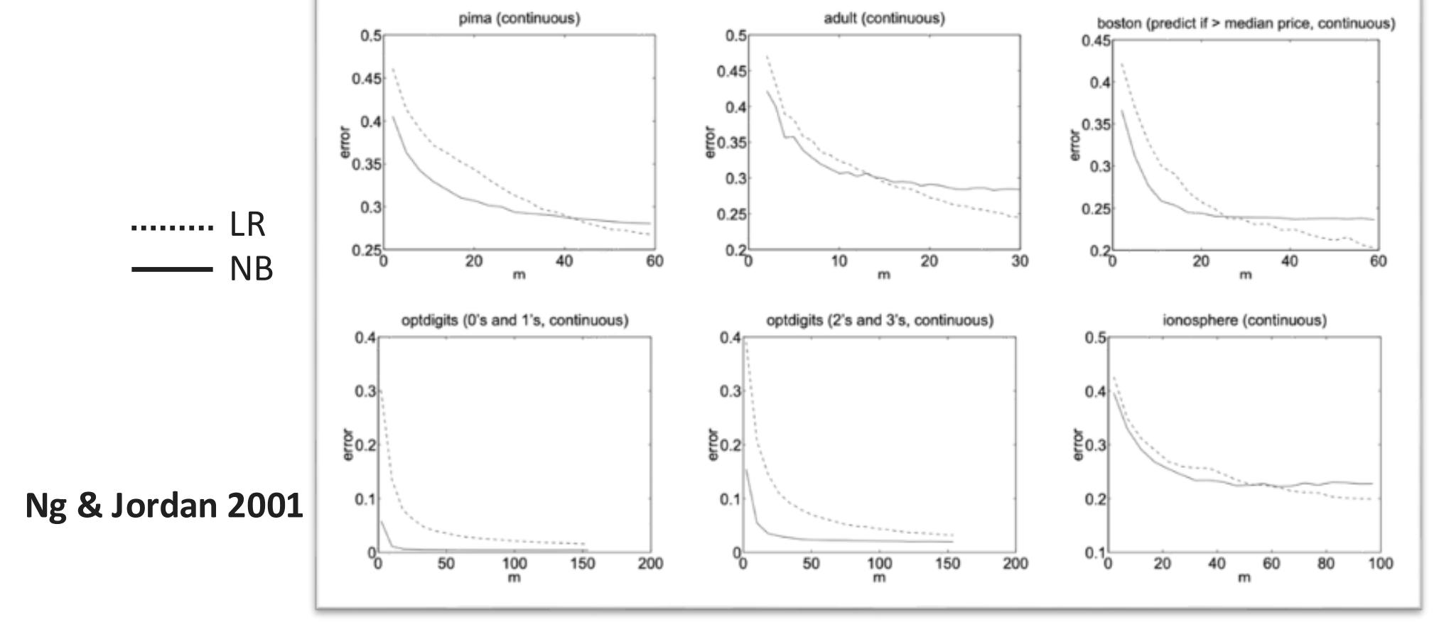
Ng and Jordan summarize the comparison as follows: “While discriminative learning has lower asymptotic error, a generative classifier may also approach its (higher) asymptotic error much faster.”
Figure 2. Learning curves of logistic regression (LR, dotted) and Naive Bayes (NB, solid).
Each panel is one UCI dataset. The horizontal axis m is the number of training examples and the vertical axis is the test error. Reproduced from Ng and Jordan (2001) as shown in the lecture slides.
On pima, adult, boston and ionosphere, Naive Bayes has the lower error when m is small, and logistic regression crosses below it as m grows. On the two optdigits tasks, Naive Bayes stays lower over the whole plotted range. In other words, the generative classifier reaches its limiting error quickly, while the discriminative classifier improves more slowly but can end up with a lower error once there is enough data.
3.4 Why? An Assumption That Does Not Always Hold
The proposition rests on an underlying assumption: generative models of the form P(X, Y; \theta) make more simplifying assumptions than discriminative models of the form P(Y \mid X; \theta). Naive Bayes, for example, assumes that the features are conditionally independent given the class (Section 2.3). When such assumptions are roughly right, they reduce the number of quantities that must be estimated, so the model needs fewer examples to reach its best performance. When they are wrong, the model keeps a bias that more data cannot remove, which is why its asymptotic error is higher.
The lecture stresses that this underlying assumption is not always true, so the proposition is not a general law. As Xue and Titterington put it, “So far there is no theoretically correct, general criterion for choosing between the discriminative and the generative approaches to classification of an observation \mathbf{x} into a class y; the choice depends on the relative confidence we have in the correctness of the specification of either p(y \mid \mathbf{x}) or p(\mathbf{x}, y) for the data.”
3.5 Modern Deep Generative Models
Modern deep generative models (DGMs) aim for generative models of the form P(X, Y; \theta)without strong simplifying assumptions, so that they can represent complex, high-dimensional observations. From here on we model the inputs alone, without labels. The key idea is a hidden (latent) structurez that explains a high-dimensional observation x. The model assumes a process that first samples z and then generates x from it:
z \sim p(z), \qquad x \sim p_\theta(x \mid z), \qquad p_\theta(x, z) = p_\theta(x \mid z)\, p(z).
Following the slides, lowercase p_\theta denotes these (typically continuous) densities. The latent structure can itself be a hierarchy z_1 \to \cdots \to z_k \to x; a single z is used here for simplicity.
Unlike the label Y earlier, z is never observed. This is the fundamental challenge, and it makes two core computations difficult:
Marginal likelihood. To evaluate how probable an observation is, we must integrate over every possible latent value:
p_\theta(x) = \int p_\theta(x, z)\, dz.
Posterior inference. Given an observation, we want to know which latent values could plausibly have produced it:
The normalizer p_\theta(x) in the posterior is exactly the integral above, so in high-dimensional models both are generally intractable to compute exactly. Each type of DGM makes a different tradeoff in how it represents the data and carries out these computations.
4. Autoencoders
4.1 Overarching Goals
The first step toward deep generative models in this part of the course is the autoencoder. Unlike the classifiers above, an autoencoder is trained with unsupervised learning: it only sees inputs x, with no labels. Its goals are
finding the subspace, or manifold, on which the data distribution lies,
visualizing data that live in high dimensions, and
sampling and generating new examples.
4.2 Encoder, Latent Representation, and Decoder
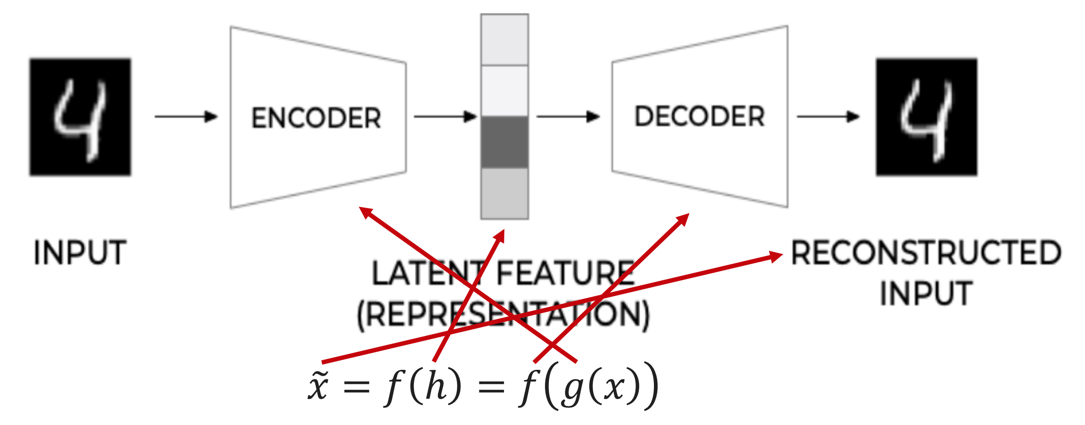
An autoencoder has two parts. The encoderg maps an input x to a latent feature representationh = g(x). The decoderf maps that representation back to a reconstructed input:
\tilde{x} = f(h) = f\big(g(x)\big).
The network is trained so that the reconstruction \tilde{x} is close to the original x. Because the latent representation h is usually much smaller than x, the network cannot simply copy its input. It has to learn a compressed description that keeps the information needed to rebuild x.
Figure 3. An autoencoder.
The encoder g compresses an input image into a latent feature representation h, and the decoder f reconstructs the input from it, \tilde{x} = f(h) = f(g(x)). The red arrows (from the lecture) link each symbol to the component it denotes: g to the encoder, h to the latent representation, f to the decoder, and \tilde{x} to the reconstruction. Adapted from Michelucci (2022) as shown in the lecture slides.
4.3 Why Reduce Dimensionality?
Learning a low-dimensional representation is useful for several reasons:
Reduce the computation cost of downstream tasks, which can work with the small representation h instead of the full input.
Improve the statistical stability of downstream tasks, since fewer dimensions means fewer quantities to estimate from the same amount of data.
Learn to generate samples. This is the idea behind variational autoencoders (Section 5.4).
Denoise observations. What if we train an autoencoder on data with intentionally added noise? Gondara (2016) does this with medical images: a convolutional autoencoder is given noisy images and learns to output clean ones. Section 5.1 describes this denoising autoencoder.
4.4 A Basic Fully-Connected Autoencoder
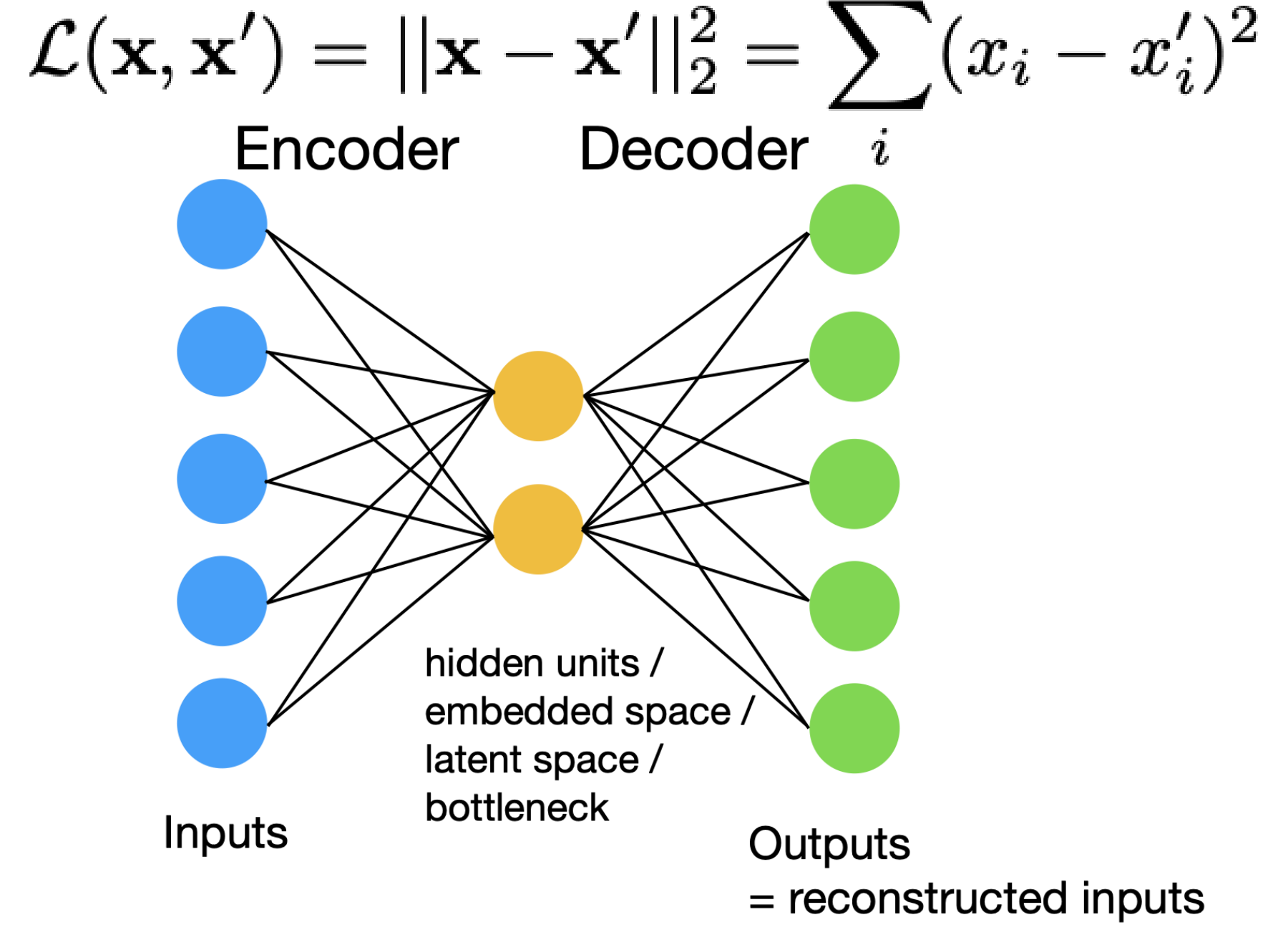
The simplest autoencoder is built from fully-connected layers, as in the multilayer perceptrons of earlier lectures. The input layer feeds a narrow hidden layer, the bottleneck, which then feeds an output layer of the same size as the input. The bottleneck units go by several names: hidden units, embedded space, latent space, or bottleneck. The outputs are the reconstructed inputs.
The network is trained to minimize the reconstruction error, the squared Euclidean distance between the input and its reconstruction:
where bold \mathbf{x} is the input vector and the sum runs over its components x_i (here i indexes input components, not training examples). (The slides write the reconstruction as \mathbf{x}' here and as \tilde{x} in Figure 3; they are the same quantity.) Because the target is the input itself, no labels are needed.
Figure 4. A basic fully-connected autoencoder.
Five inputs are compressed into a two-unit bottleneck by the encoder and expanded back to five outputs by the decoder. The network is trained with the squared reconstruction error shown on top, where \mathbf{x}' denotes the reconstruction. Figure from the lecture slides.
4.5 Using the Latent Embedding
Often the decoder is only needed during training. Once the autoencoder has been trained, we can discard the decoder and keep the encoder. The latent embedding h = g(x) then serves as a compact input for downstream machine learning tasks, such as a classifier.
5. Autoencoder Variants
The basic autoencoder can be modified to encourage representations with useful properties. Each variant below changes either the input, the network, or the loss.
5.1 Denoising Autoencoders
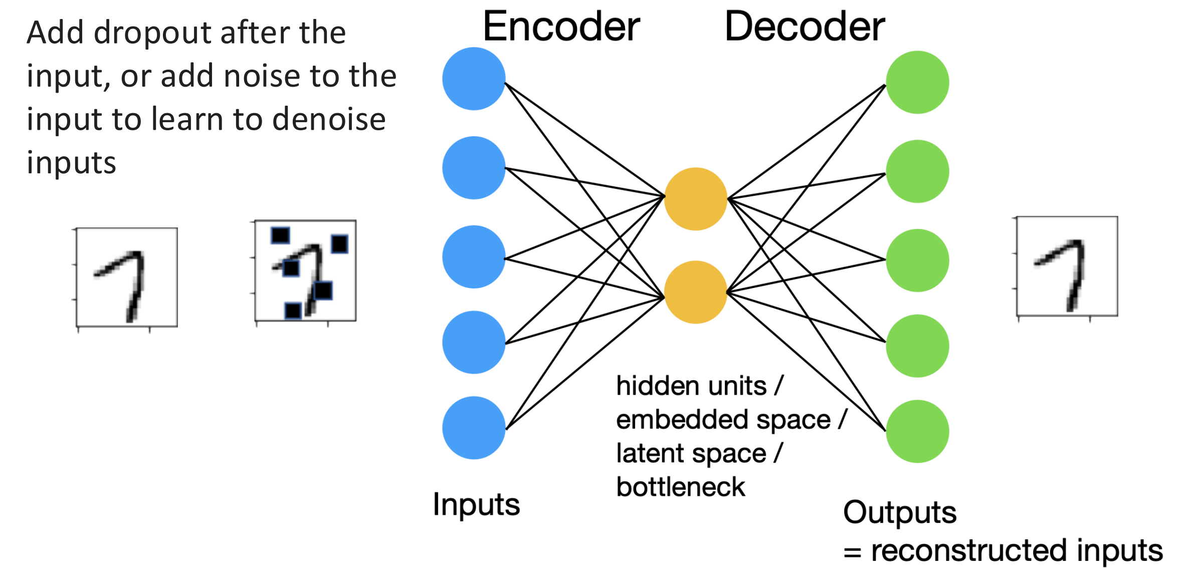
A denoising autoencoder corrupts the input during training, either by adding dropout right after the input layer (randomly setting some input values to zero) or by adding noise to the input. The training target is still the original, clean input. To reconstruct it, the network has to learn to remove the corruption, so it learns to denoise inputs.
Figure 5. A denoising autoencoder.
A clean digit (left) is corrupted by overlaying random black squares (middle) before it enters the encoder. The network is trained to output the clean digit (right). Figure from the lecture slides.
5.2 Autoencoders and Dropout
Dropout layers can also be added inside the network. As in Lecture 9, dropout randomly removes units during training, so no single unit can be relied on. This forces the network to learn redundant features that still allow a good reconstruction when some units are missing.
5.3 Sparse Autoencoders
A sparse autoencoder adds an L1 penalty on the latent representation to the reconstruction loss. Writing Enc for the encoder and Dec for the decoder (the g and f of Section 4.2), the loss is
where Enc_i(\mathbf{x}) is the i-th component of the latent representation. As with L1 regularization of weights in Lecture 9, the L1 penalty pushes many of these components to zero (or near zero), so each input is described by only a few active latent features. Sparsity is one kind of prior on the representation, just as the L1 penalty on weights corresponds to MAP estimation with a Laplace prior (Section 2.6).
Sparse representations are useful for post-hoc interpretability: because only a few features are active for any input, individual features are easier to inspect and often correspond to a single recognizable concept. A prominent example is Anthropic’s “Scaling Monosemanticity” work, which trained sparse autoencoders on the internal activations of a production large language model and extracted millions of features, many of which are interpretable (for example, a feature that responds to sycophantic praise) and can be used to steer the model’s behavior.
5.4 Preview: Variational Autoencoders
A variational autoencoder (VAE) defines the latent dimensions to follow a standard normal distribution, p(z) = \mathcal{N}(\mu = 0, \sigma^2 = 1). This is what enables sampling: to generate a new example, draw z from p(z) and pass it through the decoder. The loss for training example x^{[i]} is
Unlike the deterministic code h = g(x) of a plain autoencoder, the VAE treats the latent as a random variable z, the latent z of Section 3.5. Here q_w(z \mid x^{[i]}) is the distribution over latent codes produced by the encoder, and p_w(x^{[i]} \mid z) is the decoder’s distribution over inputs. The symbol w collects the parameters of both the encoder and the decoder and plays the role of \theta in Section 3.5. The first term is a reconstruction term: it is small when the decoder assigns high probability to the original input. The second term is the Kullback–Leibler (KL) divergence, which measures how far the encoder’s distribution is from the prior p(z) and keeps the latent codes close to a standard normal. The VAE is one way of handling the latent-variable challenges described in Section 3.5, and it is covered in detail in the next lecture.
6. Summary
Two routes to classification. A discriminative model learns P(Y \mid X) directly. A generative model learns P(X, Y) = P(X \mid Y) P(Y) and obtains P(Y \mid X) with Bayes’ theorem (Section 1).
Logistic regression vs. Naive Bayes. Logistic regression maximizes the conditional likelihood P(Y \mid X; \theta); Gaussian Naive Bayes maximizes the joint likelihood P(X, Y; \theta) under the assumption that features are conditionally independent given the class. Adding a prior P(\theta) turns maximum likelihood into MAP estimation, which is the same as adding a regularization penalty (Section 2).
Which one wins. Ng and Jordan observe that Naive Bayes can approach its (higher) asymptotic error with fewer training examples, while logistic regression improves more slowly but can reach a lower asymptotic error. This rests on the assumption that generative models make more simplifying assumptions than discriminative ones, which is not always true; there is no general criterion, and the choice depends on how confident we are that P(Y \mid X) or P(X, Y) is correctly specified. Deep generative models instead posit an unobserved latent variable z, which makes the marginal likelihood and the posterior hard to compute (Section 3).
Autoencoders. An encoder maps the input to a lower-dimensional latent representation, and a decoder reconstructs the input from it; the network is trained with a reconstruction loss. Often the decoder is discarded after training and the latent embedding is used as input for downstream tasks. A plain autoencoder is a first step toward, but not yet, a deep generative model (Section 4).
Variants. Each variant changes the input, the network, or the loss. Denoising autoencoders corrupt the input (with dropout or noise) and learn to reconstruct the clean version; dropout inside the network forces redundant features; sparse autoencoders add an L1 penalty on the latent code, a prior that favors sparse representations and aids post-hoc interpretability. The variational autoencoder, previewed in Section 5.4 and covered in the next lecture, makes the latent representation a random variable with a standard normal prior, which enables sampling (Section 5).