Lecture 14: Variational Autoencoders and Generative Adversarial Networks
An overview of VAEs, GANs, and a unified view of the two
1. Recap: Generative Models and Autoencoders
Last lecture introduced generative models, which model the joint distribution of data
Two Paths to P(Y|X)
Two ways of predicting a label $Y$ from an input $X$, given observations $X, Y$:
- Discriminative models: Learn $P(Y\mid X)$ directly.
- Generative models: Learn $P(X\mid Y)$ and $P(Y)$, then calculate:
Deep Generative Models
Deep generative models use neural networks to represent complex distributions. Multiple layers of hidden variables hope to capture the hidden structure $z$ that explains high-dimensional $X$ values.
Because we do not observe $z$, two important computations become difficult:
- Marginal likelihood:
p_\theta(x)=\int p_\theta(x,z)\,dz - Posterior inference:
p_\theta(z\mid x) \propto p_\theta(x\mid z)p(z)
Each type of deep generative model makes a tradeoff.
Autoencoders
An autoencoder consists of an encoder, which maps an input $X$ to a latent space $z$, and a decoder, which reconstructs the input from that latent space.
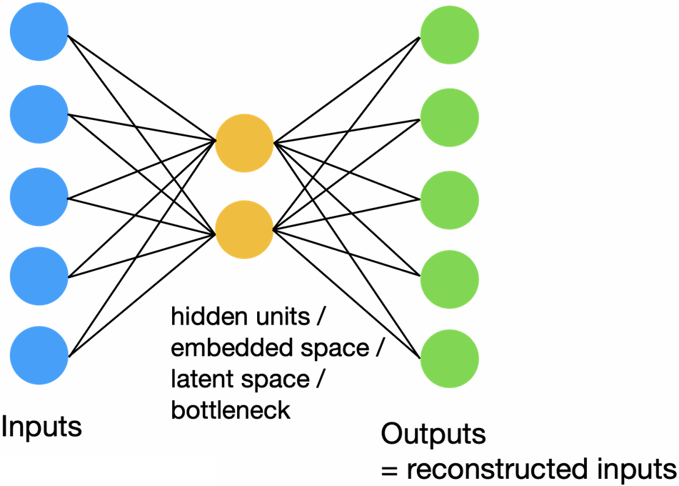
This bottleneck enables the autoencoder to capture useful structure. However, without knowing the distribution of this latent space $z$, we cannot conveniently use the autoencoder to generate new $X$: a randomly chosen $z$ may fall in a region the decoder has never learned to use.
A VAE addresses this problem by introducing a prior $p(z)$, allowing us to sample $z$ values.
2. Variational Autoencoders (VAEs)
The goal is to shape the latent space $z$ into a chosen prior distribution $p(z)$. Once the model is trained, this allows us to sample from this distribution and feed it through the decoder to generate new $x’$. This introduces a new problem: the encoder needs to learn to map inputs $x$ to our chosen latent space. To achieve this, rather than mapping each $x$ to a single point in $z$, the encoder will map inputs to conditional distributions $q(z\mid x)$ that align with our prior $p(z)$.
The Encoder: Variational Inference
We want to approximate the true posterior $p(z\mid x)$. Variational inference is a method that will allow the encoder to learn a proxy for this posterior.
The main idea is to choose a family of distributions parameterized by variational parameters $v$,
then find $v$ that minimizes the discrepancy between q and the true posterior. Restricting the distributional family to known distributions makes this feasible.
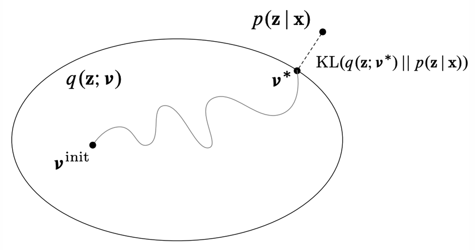
In a VAE, an encoder network, with weights $\phi$, learns the parameters of $q_{\phi}(z\mid x)$. Our measure of how close q is to the posterior of interest is the KL divergence:
The Decoder
The ideal generation process:
- $z$ is sampled from the true prior $p_{\theta^*}(z)$
- $x$ is sampled from the true conditional $p_{\theta^*}(x\mid z^{(i)})$
To represent this model, we will choose the prior $p(z)$ to be a simple distribution, such as a Gaussian. Since the conditional $p(x\mid z)$ is more complex, we will represent it with a neural network.
To train the model, we’d ideally maximize the likelihood of training data:
Bringing it Together
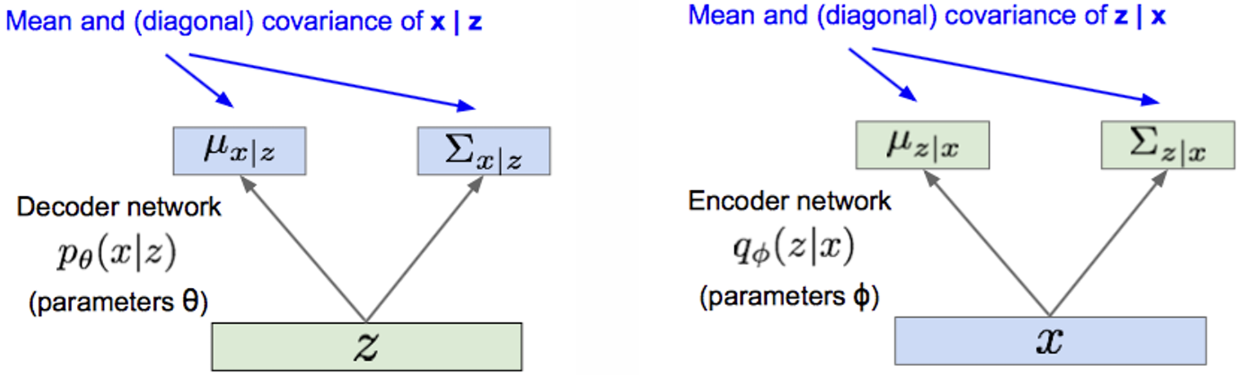
The decoder network has parameters
The encoder network has parameters
Deriving the Loss Function
Start with the log-likelihood of the observation $x$ under the model parameterized by $\theta$. We take the expectation over the posterior distribution produced by the encoder network (they are equivalent since $p_\theta(x^{(i)})$ does not depend on $z$).
The next steps are an application of Bayes’ Rule, arithmetic, and the definition of KL divergence:
This first term is the reconstruction loss. The second measures how close our learned function $q$, within the variational family, is to our chosen prior. The third term measures how far our learned function $q$ is from the true distribution $p_\theta(z\mid x^{(i)})$. We do not know $p_\theta(z\mid x^{(i)})$ so we choose to ignore it. We do know it’s nonnegative, so the first two terms form an evidence lower bound (ELBO):
Training maximizes the ELBO. The two terms serve different purposes:
- Reconstruction term: Encourages the decoder to assign high probability to the original input $x$ given its $z$.
- Prior regularization term: Penalizes the encoder distribution for being too far from the prior, helping make samples of $z$ from the prior useful for generation.
Putting it Together
Maximizing the lower bound
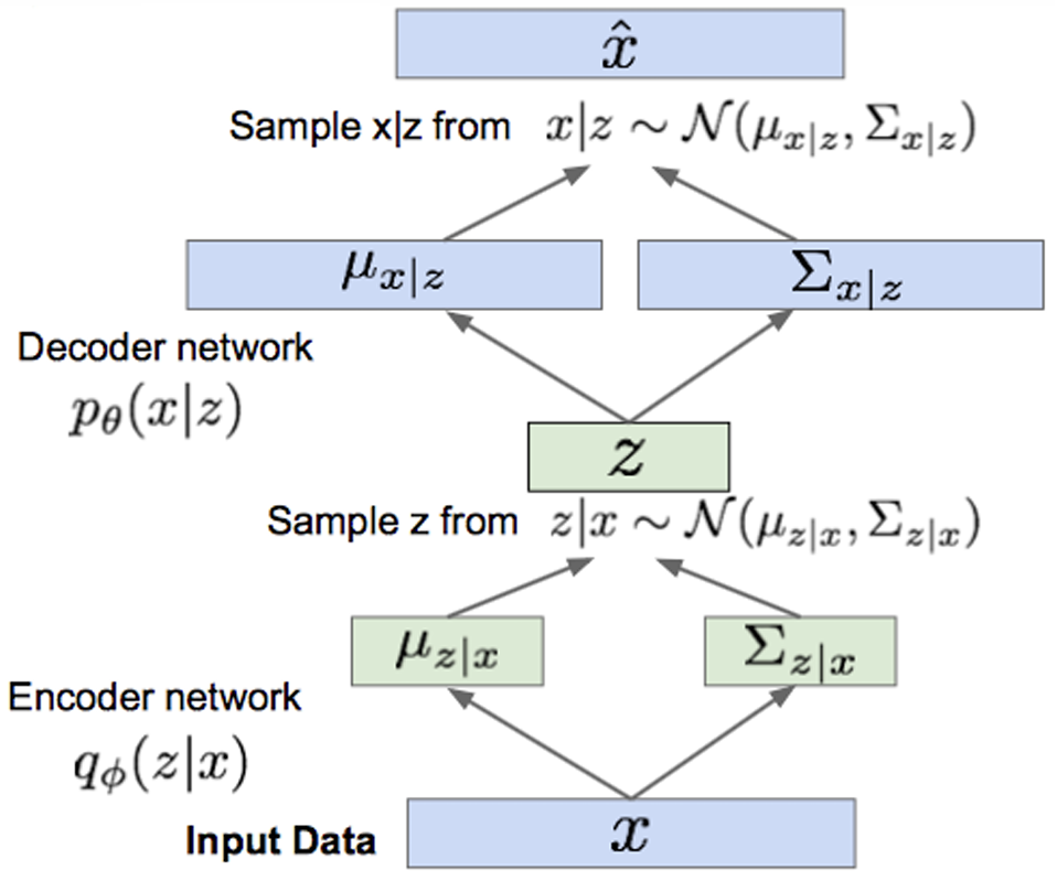
forward pass for a given minibatch:
- Start with input data $x$, pass it to encoder network
- Encoder network uses $q_\phi(z\mid x)$ to predict $\mu_{z\mid x}$ and $\Sigma_{z\mid x}$
- Sample $z$ from $z\mid x \sim \mathcal{N}(\mu_{z\mid x}, \Sigma_{z\mid x})$, pass it to decoder network
- Decoder network uses $p_\theta(x\mid z)$ to predict $\mu_{x\mid z}$ and $\Sigma_{x\mid z}$
- Sample $x\mid z$ from $x\mid z \sim \mathcal{N}(\mu_{x\mid z}, \Sigma_{x\mid z})$
Generation
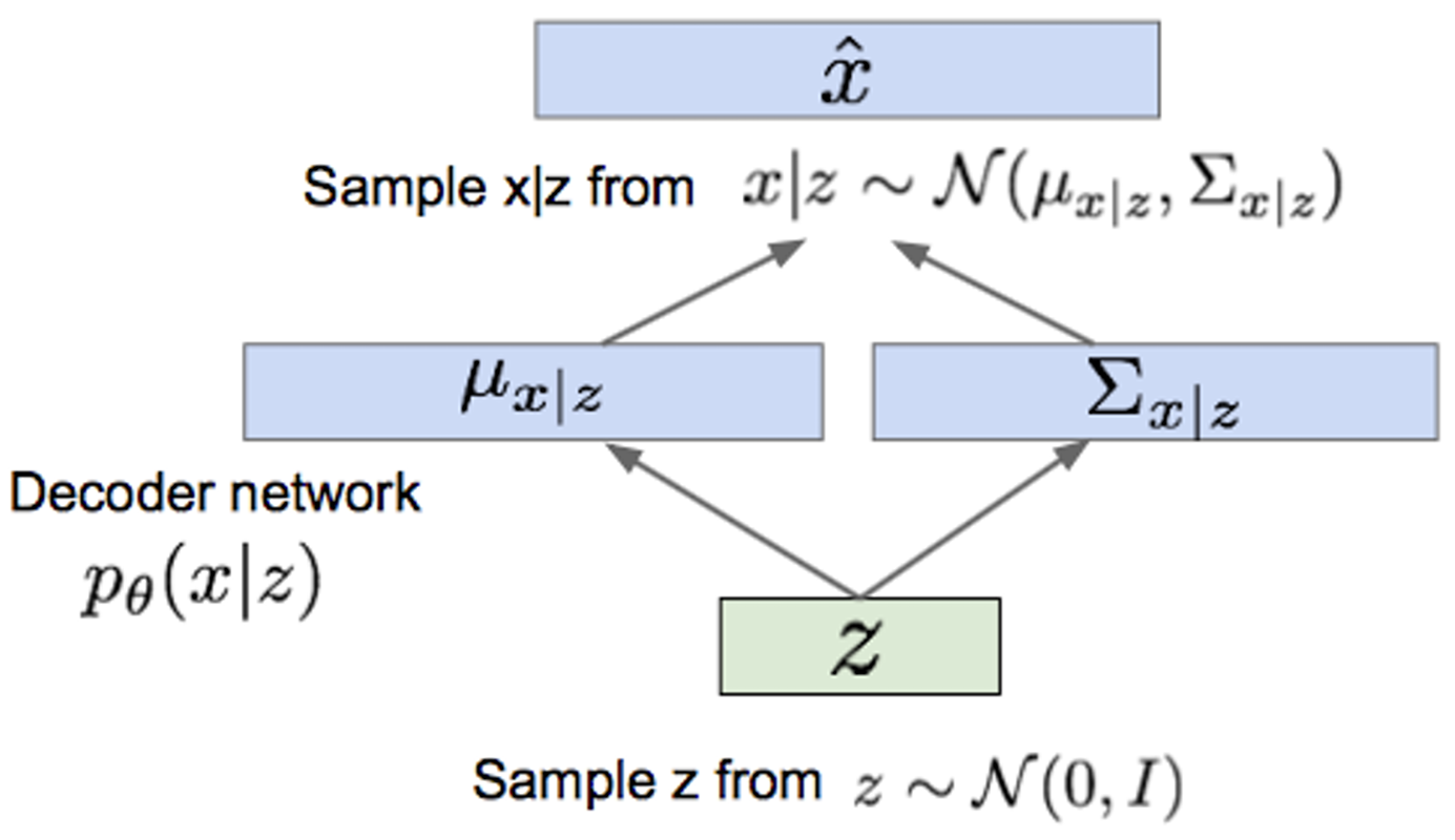
After training, generate new $x$ by sampling $z$ from the prior and use only the decoder:
Generative Adversarial Networks (GANs)
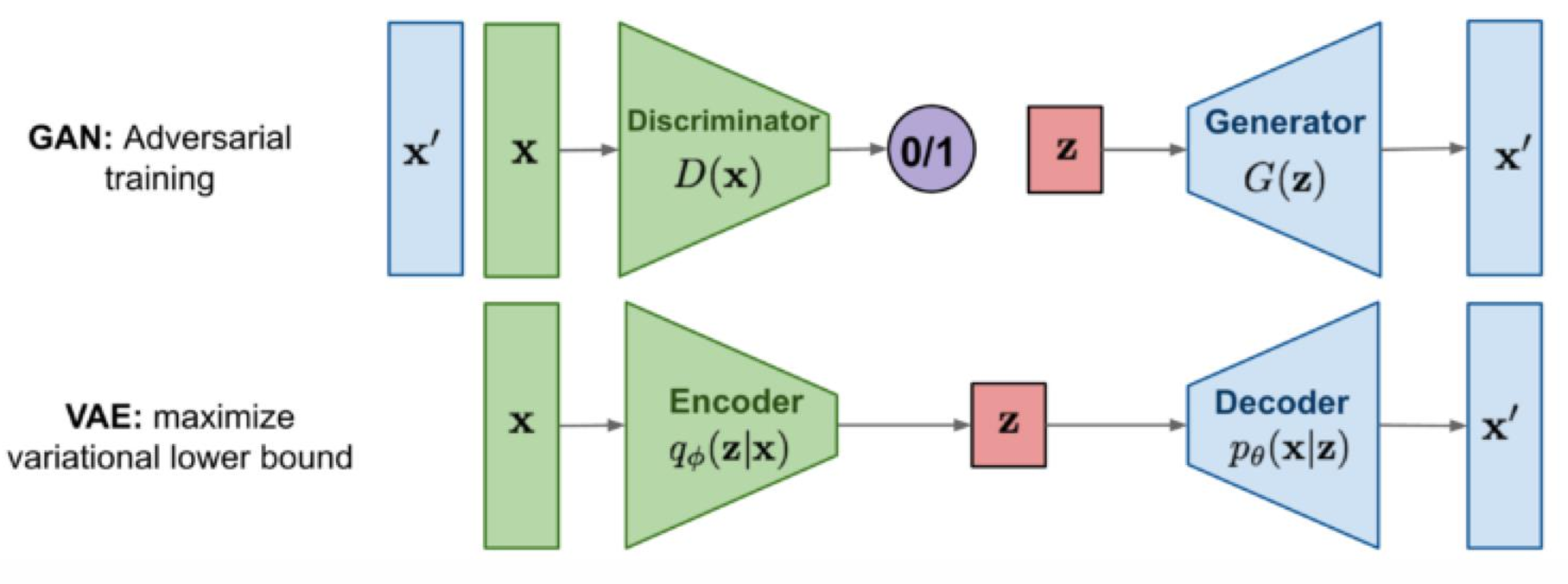
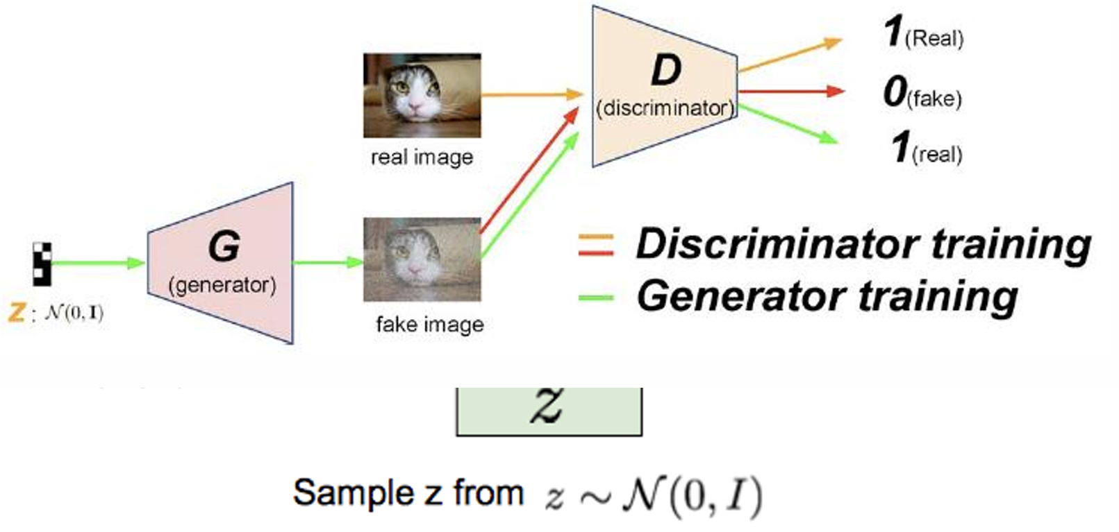
GANs learn to generate data through an adversarial game between a generator and a discriminator. The goal is to learn the training set distribution and generate new data resembling the training data. Like the VAE, GANs generate an entire image all at once, in contrast to autoregressive models or RNNs.
Discriminator and Generator
The two networks have competing roles:
- Discriminator
D(x) : Learns to become better at distinguishing real training data from generated training data. - Generator
G(z) : Learns to generate better training data to fool the discriminator.
The generator takes random noise (sampled from a known prior distribution) as input and supplies the discriminator with generated data. The discriminator assesses the generated data and then supplies the generator its loss function.
Training
Discriminator objective:
Generator objective:
Together, the GAN objective is a minimax:
The discriminator maximizes this expression, assigning high probabilities to real examples and low probabilities to generated ones. The generator minimizes it, encouraging the discriminator to assign high probabilities to its outputs.
Training alternates between two updates:
- Update the discriminator: Sample real data and sample noise to generate fake data. Maximize the real/fake classification objective while holding the generator fixed.
- Update the generator: Sample noise vectors and minimize the generator objective while holding the discriminator’s parameters fixed. Gradients pass through the discriminator into the generator.
Discriminator stochastic gradient (update by ascending):
Generator stochastic gradient (update by descending):
where
At an ideal equilibrium, the generator distribution matches the data distribution, the optimal discriminator outputs
Training Problems
GAN training can be unstable because each network changes the learning problem faced by the other.
- Oscillation: Generator and discriminator performance fluctuates rather than converging smoothly.
- Mode collapse: The generator produces only a few kinds of examples, even when training data contains many distinct kinds.
- An overly strong discriminator: Discriminator confidently rejects generated examples, leaving the generator with a vanishing gradient/the inability to keep up.
- An overly weak discriminator: Discriminator is fooled easily by unrealistic outputs and provides unhelpful learning signal (rare).
- Hyperparameter sensitivity: Generally sensitive to learning rate and other hyperparameters.
Non-saturating generator loss can help prevent vanishing gradients, ask your doctor if it’s right for you:
A Unified View (Bonus)
Both VAEs and GANs combine a process that produces observations with a process that infers something about them, but their objectives and network roles differ.
GANs: Rewritten
Consider an implicit distribution over $x\sim p_\theta (x\mid y)$ with a binary label
The generated data is sampled via
then the objectives become
These objectives maximize the conditional log-likelihood of $y$ with the distribution $q_\phi (y\mid x)$ conditioned on data/generated data $x$ from $p_\theta (x\mid y)$. Here, $q_\phi (y\mid x)$ is the generative model and $p_\theta(x\mid y)$ is the inference model.
Compare these to the reconstruction term of a VAE’s ELBO. In a VAE, this term serves to maximize the conditional log-likelihood of $x$ with the generative distribution $p_\theta (x\mid z)$ conditioned on the latent code $z$ inferred by $q_\phi (z\mid x)$. From earlier, we know $p_\theta (x\mid z)$ is the generative model and $q_\phi (z\mid x)$ is the inference model.
VAEs vs GANs
- VAE reconstruction: Predict the observation
x given an inferred latent codez . - GAN discrimination: Predict the source label
y given an observed or generated examplex .
Side-by-side
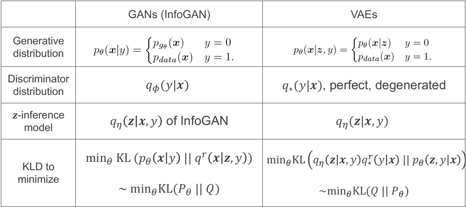
Note the asymmetry in KL divergence minimization: GANs minimize
Mode Covering vs Mode Choosing
Mode Covering vs. Mode Choosing
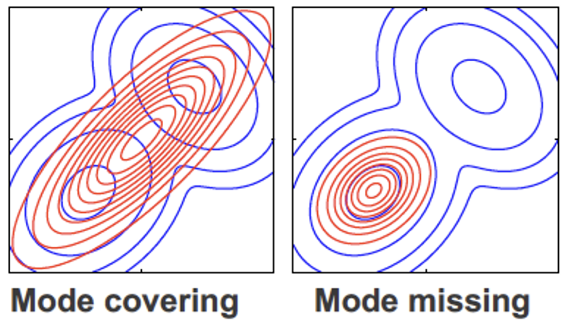
Models balance producing realistic examples with representing the diversity of the data. VAEs tend to cover modes: rather than commit to generating only the most realistic data, their distribution spreads out to cover many modes, including regions with small values of $p_{\text{data}}$. In the case of image generation, VAEs often produce varied but blurry images, although this blurriness is also influenced by their reconstruction loss. GANs, on the other hand, tend to miss modes, choosing to include some and not others in their generation. In the case of image generation, this often results in sharper but less diverse images.
One way to conceptualize this is through their training. A GAN’s generator gets to choose which images it sends to the discriminator; once it has learned which images best fool the discriminator, why branch out to represent rarer data? VAEs, however, are evaluated based on their ability to reconstruct every image in the training data, encouraging them to represent the entire distribution rather than concentrate on a few modes.
This behavior is captured by the asymmetry of the two models’ KL divergence:
- Mode Covering: Minimizing
\text{KL}(Q\|P_\theta) strongly penalizes assigning little model probability where data occur. A limited model may spread probability across several modes, including low-density regions between them. - Mode Choosing: Minimizing
\text{KL}(P_\theta\|Q) strongly penalizes placing model probability where the data density is small. A limited model may concentrate on one mode and miss others.
What to Remember
- VAEs: Train an encoder and decoder jointly by maximizing an ELBO, balancing reconstruction likelihood with latent prior regularization. Mode covering.
- VAE generation: Sample a $z$ from the prior and run the decoder; the encoder is needed for inference, not for generating a new example.
- GANs: Train a generator to fool a discriminator that learns to distinguish real from generated examples. Mode choosing.
- GAN optimization: Alternate network updates, many potential training problems.