Lecture 15: Diffusion Models
Learning to generate images by reversing noise, from pixel-space diffusion to text-conditioned latent diffusion.
1. From reconstructing images to generating them
A classifier answers a question about an observed image, such as whether it contains a cat. A generative model instead describes a distribution from which new images can be sampled. In supervised problems this may mean modeling the joint distribution of images and labels; for unconditional image generation, the target is simply the image distribution
The lecture begins by revisiting three constructions:
- An autoencoder maps an image through an encoder and decoder,
\hat x=D(E(x)) . Reconstruction alone does not ensure that arbitrary latent vectors decode to plausible images. - A variational autoencoder (VAE) specifies a prior and a probabilistic decoder. An approximate posterior makes its likelihood objective tractable through a variational bound. Sampling starts with a draw from the prior.
- A generative adversarial network (GAN) learns a generator through a discriminator’s feedback. Its usual training objective compares generated and real samples without evaluating the image likelihood.
Diffusion offers another route: deliberately corrupt training images through a known process, and learn transitions that run in the opposite direction. A complicated image-generation problem becomes many local denoising problems. Sohl-Dickstein et al. introduced this construction; DDPMs developed a particularly effective Gaussian formulation.
Scope. These notes follow the October 29 lecture slides, particularly slides 4-20. Sections 2-3 formalize the diagrams in the lecture. The closed-form derivations in Sections 4-5 and the optional score interpretation are reading supplements, included to make the training procedure understandable without returning to the slides.
2. The forward process: destroy structure in controlled steps
Let
Here
with independent noise at each step. Multiplying the previous signal by
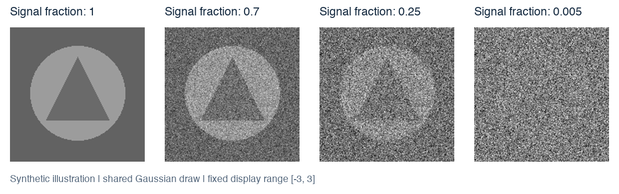
Sampling any noise level directly
Define
To check the variance, suppose the accumulated noise at step
This identity is crucial for efficient training: one can create a noisy example at a randomly selected step without simulating all preceding steps. The single
If the schedule makes
3. The reverse process: learn a distribution over cleaner images
Knowing how to add noise does not tell us how to remove it from an unknown image. By Bayes’ rule,
The marginal distributions in this expression depend on the unknown data distribution. Moreover, several plausible clean images can correspond to a similar noisy observation. Reversal therefore requires learning a conditional distribution, rather than algebraically undoing an individual noise draw.
The model starts from
We use a fixed time-dependent variance for this exposition. Other models may learn the covariance. The Gaussian transition is a modeling choice motivated by small forward steps; the exact reverse conditional need not be Gaussian for an arbitrary data distribution and finite step size.
A shared neural network receives both
The model’s image density is obtained by integrating out the noisy states:
Generation uses only the learned reverse chain. Draw a fresh
4. Why training reduces to predicting noise
The lecture’s summary links a variational bound with weighted denoising loss. The following derivation supplies the intermediate steps, using the DDPM parameterization.
A tractable training target
Although
There is no contradiction:
The variational bound
For a fixed training image, Jensen’s inequality gives a lower bound on
Rearranging the chain factors separates three kinds of terms:
The first term measures terminal-prior mismatch and is constant with respect to
For fixed
Predict noise instead of the reverse mean
Use the forward equation to express
Thus the network predicts the accumulated noise, and a known formula converts that prediction into a reverse mean. Substitution into the preceding squared error gives, for
Here
Here the image is sampled from the data distribution, the timestep uniformly from
This is supervised regression with targets generated automatically from the data. It is a reweighted training objective, not literally the exact NLL or the complete variational bound. The
Optional reading connection: the score
The score is the gradient of a log density with respect to its input. For the forward conditional Gaussian,
At the population squared-error optimum, the noise predictor estimates
5. Training and sampling are different computations
One training update samples clean images, timesteps, and Gaussian noise, then regresses the predicted noise toward the sampled noise. For batch size
Training update:
    sample a batch of clean images x0
    independently sample one timestep t and Gaussian noise epsilon per image
    xt = sqrt(alpha_bar[t]) * x0 + sqrt(1 - alpha_bar[t]) * epsilon
    prediction = noise_network(xt, t)
    loss = batch_mean(sum_over_image_coordinates((epsilon - prediction)^2))
    backpropagate loss and update network parameters
After training, a basic ancestral sampler uses the reverse mean from Section 4:
Sampling (one simple DDPM convention):
    x = sample_standard_normal(image_shape)
    for t = T, T-1, ..., 1:
        prediction = noise_network(x, t)
        mean = (x - beta[t] / sqrt(1 - alpha_bar[t]) * prediction)
               / sqrt(alpha[t])
        if t > 1:
            x = mean + sqrt(beta_tilde[t]) * sample_standard_normal(image_shape)
        else:
            x = mean
    return x
This convention uses posterior variance
Training needs only a randomly chosen noise level per example; the basic sampler requires a sequence of network evaluations. That distinction explains why a simple denoising training objective can still lead to expensive generation.
6. Latent diffusion: move the repeated computation out of pixel space
Large images make every denoising evaluation expensive. The lecture therefore asks whether diffusion should run directly on pixels. A latent diffusion model first learns a useful compressed representation with an autoencoder, then models the distribution of those representations.
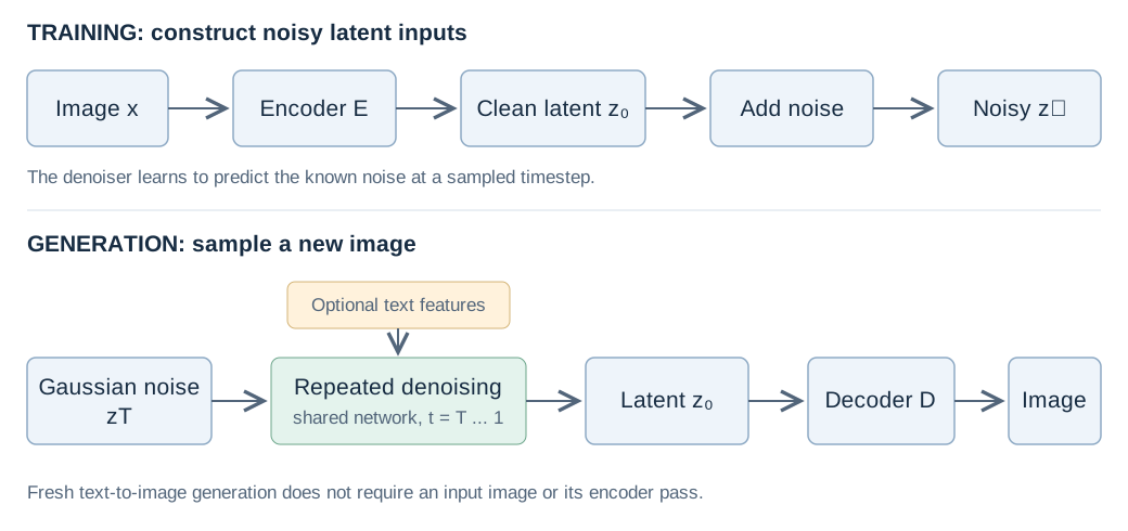
Write
Generation draws
For a dimensional illustration, compressing an RGB
Rombach et al. develop this separation between perceptual compression and generative modeling, including conditioning through cross-attention.
7. Text conditioning and the Stable Diffusion idea
Unconditional diffusion samples from a general learned image distribution. Text-to-image generation instead aims at a conditional distribution,
The corresponding training target is still the known noise. What changes is the information available to predict it. In a cross-attention implementation, queries come from image features and keys and values come from text features, letting spatial image features attend to prompt tokens.
At generation time, encode the prompt, draw latent Gaussian noise, run the text-conditioned denoising chain, and decode the final latent. This is the combination emphasized by the lecture’s Stable Diffusion slides: compressed image representations plus iterative denoising plus text conditioning. It describes the latent-diffusion architecture discussed in class, without assuming that all image-generation products or model versions use the same internal design.
8. Comparing VAE, GAN, and diffusion objectives
| Property | VAE | GAN | Diffusion |
|---|---|---|---|
| Construction | Prior, decoder likelihood, approximate encoder posterior | Prior and generator, trained against a discriminator | Fixed corruption process, prior, learned reverse transitions |
| Training signal | Reconstruction likelihood and posterior-prior KL | Adversarial discrepancy between real and generated samples | Variational bound or a reweighted denoising objective |
| Likelihood treatment | Optimize an evidence lower bound | Standard objective does not evaluate likelihood | Bound the likelihood; simple noise MSE changes the weighting |
| Basic generation path | Sample latent, decode | Sample latent, run generator | Sample noise, repeatedly denoise; decode if latent-based |
| Typical concern | Posterior approximation and reconstruction quality | Training instability and mode collapse | Sequential sampling cost and schedule/model approximation |
The lecture’s labels such as VAE blurriness, GAN realism, or diffusion mode coverage summarize tendencies rather than universal guarantees. Architecture, data, objective, and inference choices affect quality and diversity. A likelihood-based construction does not by itself prove that every data mode will be represented by a fitted model.
9. Checks for understanding
- Which direction is learned? The reverse transitions are learned. In the formulation here, the forward variance schedule is fixed.
- Why can training skip forward steps? Gaussian composition gives the closed-form marginal
q(x_t\mid x_0) . - Why can we compute a posterior target but still need a network? The tractable target also conditions on the training image
x_0 , which is unavailable during generation. - Is noise MSE the exact likelihood objective? No. It is a useful reweighting; the full variational bound also contains terminal and reconstruction terms.
- What does latent diffusion change? The space in which the chain operates. It still requires learning denoising transitions.
- What does text conditioning change? The reverse prediction can depend on a prompt, so samples target a conditional image distribution.
The central construction is to learn generation through a sequence of manageable conditional predictions. The forward process supplies noisy inputs and known training targets; the learned reverse process turns fresh noise into new samples.