Lecture 16: Sequence Learning with RNNs
Turning words into vectors, recurrent neural networks and their variants, backpropagation through time and why its gradients vanish or explode, LSTMs and GRUs, and why recurrence has come back in modern sequence models.
Scope. These notes follow the November 3 lecture slides
Notation. We write
1. Two Challenges with Text
In the diffusion lecture, a text prompt conditioned the image generator. That raised a question the lecture left open: how does a sentence become numbers that a network can use? Text poses two separate problems
- Turning words into numbers. We need a representation of words through which activations can flow forward and gradients can flow backward.
- Modeling sequences. Sentences have different lengths, and a word can depend on another word far away from it. A model should accept variable-length input and carry context across long ranges.
The rest of the module maps onto these problems. This lecture handles variable-length input with RNNs. Attention and transformers (Lecture 17) address long-range dependencies. GPT architectures (Lecture 18) give a generative model of text, and the remaining lectures cover scale, alignment, reasoning and parameter-efficient fine-tuning.
Where the module is going. GPT is an autoregressive probabilistic model
Here
2. Three Classic Ways to Avoid the Sequence Problem
Before RNNs, the common approaches did not solve the sequence problem; each made a simplifying assumption that removed it.
2.1 Bag-of-Words: Discard the Order
Build a vocabulary, then represent each document by how many times each word occurs. With the vocabulary and=0, is=1, one=2, shining=3, sun=4, sweet=5, the=6, two=7, weather=8, the three training sentences on the slide become rows of a design matrix:
| Sentence | Count vector |
|---|---|
| “The sun is shining” | [0, 1, 0, 1, 1, 0, 1, 0, 0] |
| “The weather is sweet” | [0, 1, 0, 0, 0, 1, 1, 0, 1] |
| “The sun is shining, the weather is sweet, and one and one is two” | [2, 3, 2, 1, 1, 1, 2, 1, 1] |
Any classifier, such as logistic regression or an MLP, can be trained on this
2.2 Hidden Markov Models: Remember Only the Last State
A hidden Markov model assumes the hidden state at each step depends only on the previous state, and each observation depends only on the current state. The slide’s example has hidden weather (rainy or sunny) that follows a Markov chain, and observed activities (walk, shop, clean) that depend on the weather of that day. The Markov assumption removes the need to look further back. Information from many steps ago survives only if it is encoded in the current discrete state, which requires an exponentially large state space for rich histories.
2.3 Convolutional Networks: Assume a Maximum Length
A one-dimensional CNN slides filters over the sequence. It needs inputs of a fixed size, so every sentence is padded to a maximum length. This assumes a reasonably short maximum exists; longer inputs must be truncated, and each output only sees the positions within its receptive field.
3. Word Embeddings: From Words to Vectors
The first challenge is solved in two steps.
Step 1: map each word to an index. Add two special tokens to the vocabulary: <unk> for words not in the vocabulary and <pad> for padding. With <unk>=0, and=1, is=2, one=3, shining=4, sun=5, sweet=6, the=7, two=8, weather=9 and <pad>=10, “The sun is shining” becomes [7, 5, 2, 4, 10, 10, …], padded to the length of the longest sentence in the batch.
Step 2: map each index to a dense vector. Write index 7 as a one-hot vector
The slide leaves an open question: where does
Supplement. In practice no one forms the one-hot vector. torch.nn.Embedding(num_embeddings=11, embedding_dim=4) stores
4. Recurrent Neural Networks
4.1 Order Matters
The two “movie” sentences in Section 2.1 show that a sequence model must read words in order and remember what it has read. A feedforward network maps
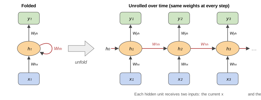
Weight sharing is what solves the variable-length problem. A five-word sentence and a five-hundred-word sentence are processed by the same parameters; the longer one simply runs the recurrence more times. It also builds in an assumption: the rule for updating the state is the same at every position.
4.2 The Equations
A single-layer RNN has three weight matrices, shared across time:
The hidden activation
Parameter count. The hidden layer has nn.RNN(4, 3) reports 27 because it keeps two bias vectors, one for the input term and one for the recurrent term, which are redundant mathematically.
A worked example. Take one hidden unit with
The input seen at step 1 still affects the state at step 3, but the trace shrinks at every step because it is multiplied by 0.8 and passed through
4.3 Multilayer RNNs
RNN layers can be stacked. The hidden state of layer 1 at time
4.4 Bidirectional RNNs
A bidirectional RNN runs one RNN from left to right and a second, separate RNN from right to left, then concatenates their states at each position:
Every output now depends on the whole sequence. In “The movie my friend has not seen is good”, the representation of “seen” can use the words “is good” that come after it. This makes bidirectional RNNs a good fit for encoding an input that is fully available: tagging each word, classifying a sentence, or the encoder of a translation model (the attention examples in the next lecture use one). They cannot generate text, because when the model produces token
4.5 Types of Sequence Tasks
Recurrence allows several input-output patterns:
| Pattern | Input and output | Example |
|---|---|---|
| Many-to-one | A sequence in, one fixed-size vector out | Sentiment analysis: text in, class label out |
| One-to-many | One input (not a sequence) in, a sequence out | Image captioning: image in, sentence out |
| Many-to-many, direct | One output per input step | Video captioning frame by frame; tagging each word |
| Many-to-many, delayed | Read the whole input, then produce an output sequence | Machine translation |
4.6 Encoder–Decoder (seq2seq)
The delayed many-to-many pattern is implemented with two RNNs
- The encoder RNN reads the four input words. Its last hidden state
c=h_4 is a fixed-length summary of the whole sentence. - The decoder RNN starts from
c and writes the output one token at a time, feeding each output token back in as the next input: from the start token<s>it produces “Dónde”, then “está”, “la”, “biblioteca” and finally the end token<eos>. - Because the decoder decides when to stop, input and output lengths can differ. The same design serves translation, summarization and question answering.
The weakness is a bottleneck: everything the decoder knows about the source must fit into one fixed-length vector
Supplement. During training the decoder is usually fed the correct previous target word rather than its own prediction (“teacher forcing”), which lets all decoder steps be trained from the reference translation. At test time the decoder only has its own predictions, so early mistakes can compound. The mismatch between the two conditions is known as exposure bias.
5. Backpropagation Through Time
5.1 The Gradient
To train an RNN we unroll it over the
The unrolled network is an ordinary computation graph, so backpropagation applies unchanged; applied to an unrolled RNN it is called backpropagation through time (BPTT)
where
This product is straightforward to compute, and it is where the trouble starts.
5.2 Why Gradients Vanish or Explode
For a
A signal from step NaN. The same problem appeared for deep feedforward networks in Lecture 7, but here it is worse: an RNN on a 100-word sentence is 100 layers deep with the same matrix at every layer, and dependencies across sentences require far more steps.
Supplement (Pascanu et al., this week’s reading). The scalar intuition can be made precise
If
Figure 3 (in Section 6.4) shows these regimes in an actual randomly initialized network with 64 hidden units. With all singular values of
5.3 Fixes
Gradient clipping. If the norm of the gradient exceeds a threshold, rescale the gradient down to that norm while keeping its direction. For example, a gradient of norm 50 with threshold 5 is multiplied by
loss.backward()
torch.nn.utils.clip_grad_norm_(model.parameters(), max_norm=5.0)
optimizer.step()
Truncated backpropagation through time (TBPTT). Limit how many steps the gradient can travel back after each forward pass. A sequence may have 100 steps while gradients are propagated through only the last 20 or so. This bounds the length of the Jacobian product and the memory needed for stored activations. The cost is that the model cannot learn, through gradients, dependencies longer than the window, although the hidden state itself still carries information forward. In PyTorch, TBPTT means splitting a long sequence into chunks and calling h = h.detach() between chunks, so the value of the state is kept but the gradient stops there.
Change the architecture. The third fix, and the one that addresses vanishing gradients, is to give the memory a path along which the gradient is not multiplied by
6. Long Short-Term Memory (LSTM)
6.1 Two Paths of Memory
The name is not an oxymoron. An LSTM
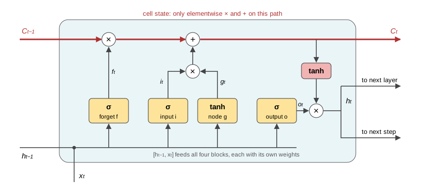
6.2 Gates and Updates
A gate is a sigmoid layer. Its output lies between 0 and 1 and says how much of something to let through: 0 blocks everything, 1 keeps everything. A
The cell state and hidden state are then updated as
The first term of
A worked example. For a single unit, suppose
The cell kept 90% of its old memory and wrote only a little new content; the output gate exposed half of the result.
6.3 Why the Cell State Helps the Gradient
Differentiate the cell update along the cell-state path only, holding the gates fixed:
Compare this with the plain RNN’s factor
6.4 Measuring It
Figure 3 measures these Jacobians directly in randomly initialized networks with 64 hidden units and random inputs. For the plain RNN we compute
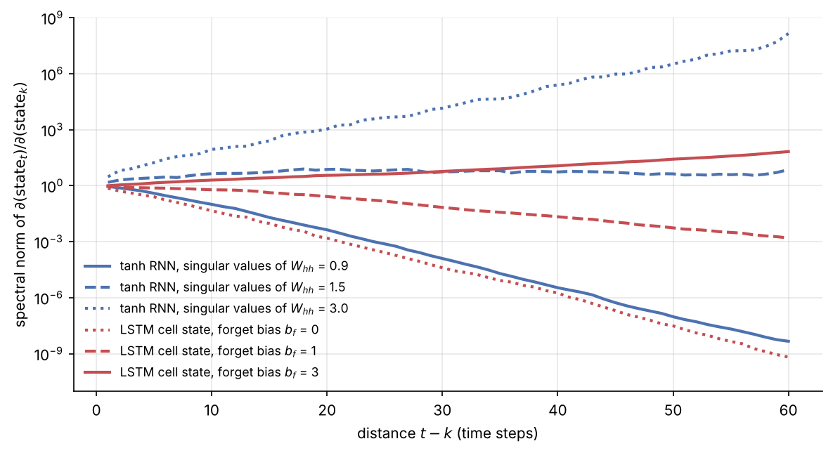
Three observations follow. First, the LSTM is not automatically immune: with forget bias 0 the forget gates sit near
Supplement. The original 1997 LSTM had no forget gate; its cell simply accumulated,
As the slides note, gating slows the decay but does not remove it; long-range gradients still fade, only more slowly. This is one of the reasons discussed in Section 8.
6.5 LSTMs in PyTorch
The slide’s example:
import torch
import torch.nn as nn

rnn = nn.LSTM(10, 20, 2)            # input_size=10, hidden_size=20, num_layers=2
input = torch.randn(5, 3, 10)       # (seq_len, batch, input_size)
h0 = torch.randn(2, 3, 20)          # (num_layers, batch, hidden_size)
c0 = torch.randn(2, 3, 20)
output, (hn, cn) = rnn(input, (h0, c0))
# output: (5, 3, 20)  top layer's h_t at every step
# hn, cn: (2, 3, 20)  every layer's state at the last step
Two details cause most shape bugs. The default batch_first=False puts the sequence dimension first, so (5, 3, 10) is 5 time steps of a batch of 3. The initial states are indexed by layer first. With bidirectional=True, the last dimension of output doubles to 40 and the first dimension of h0 and c0 becomes num_layers * 2 = 4. Other options are bias, dropout (applied between stacked layers, not after the last one) and proj_size.
Parameter count. Each of the four blocks has an weight_ih_l0 of shape weight_hh_l0 of shape nn.LSTM(10, 20) this is
7. Gated Recurrent Unit (GRU)
The GRU
The update gate
With three weight blocks instead of four, a GRU has about 25% fewer parameters than an LSTM of the same size (1920 versus 2560 for input size 10 and hidden size 20 in PyTorch), and its accuracy is usually similar torch.nn.GRU has the same interface as nn.LSTM without the cell state. One trap when reading the documentation: PyTorch swaps the roles of
8. Why RNNs Faded, and Why Recurrence Is Back
8.1 Why Transformers Replaced RNNs
- Training is sequential.
h_t cannot be computed untilh_{t-1} is done, so a length-T sequence isT dependent steps and a GPU cannot parallelize across time. A transformer processes allT positions of a training sequence at once. - Memory bottleneck. The entire past is squeezed into one fixed-size vector
h_t , the same problem as the seq2seq vectorc . Attention can look back at any earlier token directly. - Long-range gradients still fade, even with LSTM gating, just more slowly.
The net effect is that transformers turned more data and compute into better models (BERT, GPT; from 2018 onward), and by about 2020 RNNs had mostly disappeared from frontier language modeling. The slide’s summary: transformers won on training parallelism, and they pay for it at inference time.
8.2 The Cost of Attention
When a transformer generates text, every new token attends to every previous token. Generating
8.3 Linear Recurrence: Parallel Training, Recurrent Inference
The trick that brings recurrence back is to remove the nonlinearity between time steps:
(Here
Supplement: why linearity allows a parallel scan. Consider the scalar case and write
Timeline. Linear attention
Today: hybrids. Current models such as Jamba (2024), Nemotron-H and Qwen3-Next (2025) use mostly recurrent layers plus a few attention layers.
Why keep any attention? A fixed-size state cannot store everything. Exact recall and copying from long contexts remain hard for purely recurrent models
9. Checks for Understanding
- Why can one RNN process sentences of any length? The same weights
W_{hx}, W_{hh}, W_{yh} are applied at every step; a longer sentence only runs the recurrence more times. - How many parameters does the hidden layer of a plain RNN with
d=10 ,n=20 have?nd+n^2+n = 200+400+20 = 620 (640 in PyTorch, which keeps two bias vectors). An LSTM has four blocks and a GRU three. - Why can a bidirectional RNN not generate text? Its backward direction reads tokens that come later, which do not exist yet during generation.
- What limits a seq2seq model with a single context vector? All information about the input must pass through one fixed-length vector
c , which loses detail on long inputs. - Why do gradients vanish or explode in BPTT? The gradient across
t-k steps is a product oft-k Jacobians\mathrm{diag}(1-h_i^2)W_{hh} ; its norm behaves roughly like a number raised to the powert-k . - Does gradient clipping fix vanishing gradients? No. It only rescales gradients that are too large.
- Why does the LSTM’s cell state help? Along the cell path, each step multiplies the gradient only by the forget gate, which the network can keep near 1, instead of by
W_{hh} and a\tanh derivative. - What is the trade-off between transformers and recurrent models? Transformers train in parallel but cost
O(T^2) attention and a growing cache at inference; recurrent models keep anO(1) state per token. Linear recurrences get both parallel training and recurrent inference.
10. Key Takeaways
- Text needs a numeric representation (vocabulary index, then a learned embedding vector) and a model that handles variable-length sequences.
- An RNN reuses one set of weights at every step and carries a hidden state
h_t=\tanh(W_{hx}x_t+W_{hh}h_{t-1}+b_h) , so it handles any length with a fixed number of parameters. - Stacked, bidirectional and encoder–decoder RNNs cover classification, tagging, captioning and translation. Bidirectional models only encode, and seq2seq compresses the input into one vector.
- Backpropagation through time multiplies one Jacobian per step, so gradients vanish or explode over long ranges. Clipping fixes exploding gradients; truncated BPTT limits how far gradients travel.
- The LSTM’s additively updated cell state, controlled by forget, input and output gates, lets gradients survive many steps; the GRU achieves a similar effect with two gates and about 25% fewer parameters.
- Transformers replaced RNNs because they train in parallel. Linear recurrences (S4, Mamba, xLSTM) and hybrid models bring recurrence back for cheap long-context inference, while a few attention layers keep exact recall.
Further reading. Karpathy’s blog post