Lecture 04
Single-layer networks
Announcements
- HW1 Due this Friday (Sep 19), submit your HW via Canvas.
- If you are still on the waitlist for this course and waiting nervously, please send an email to Prof. Lengerich.
Outline
- Perceptrons
- Geometric intuition
- Notational conventions for single-layer nets
- A fully-connected (linear) layer in PyTorch
1. Perceptrons
Rosenblatt’s Perceptron
First, we’ll talk about Rosenblatt’s perceptron, which is seen as the foundation of today’s artificial neural networks.
What Rosenblatt proposed is actually “A learning rule for the computational/mathematical neuron model”. This contains two parts:
- A computational/mathematical neuron model,
- A learning rule.
So back to 1957, Rosenblatt not only defined the mathematical model for an artificial neuron (weighted sum + activation function), but also formulated a learning rule that enables the model to learn autonomously from data.
In our brain, there are lots of neurons. Similarly, we invented artificial neural networks to mimic this biological structure.
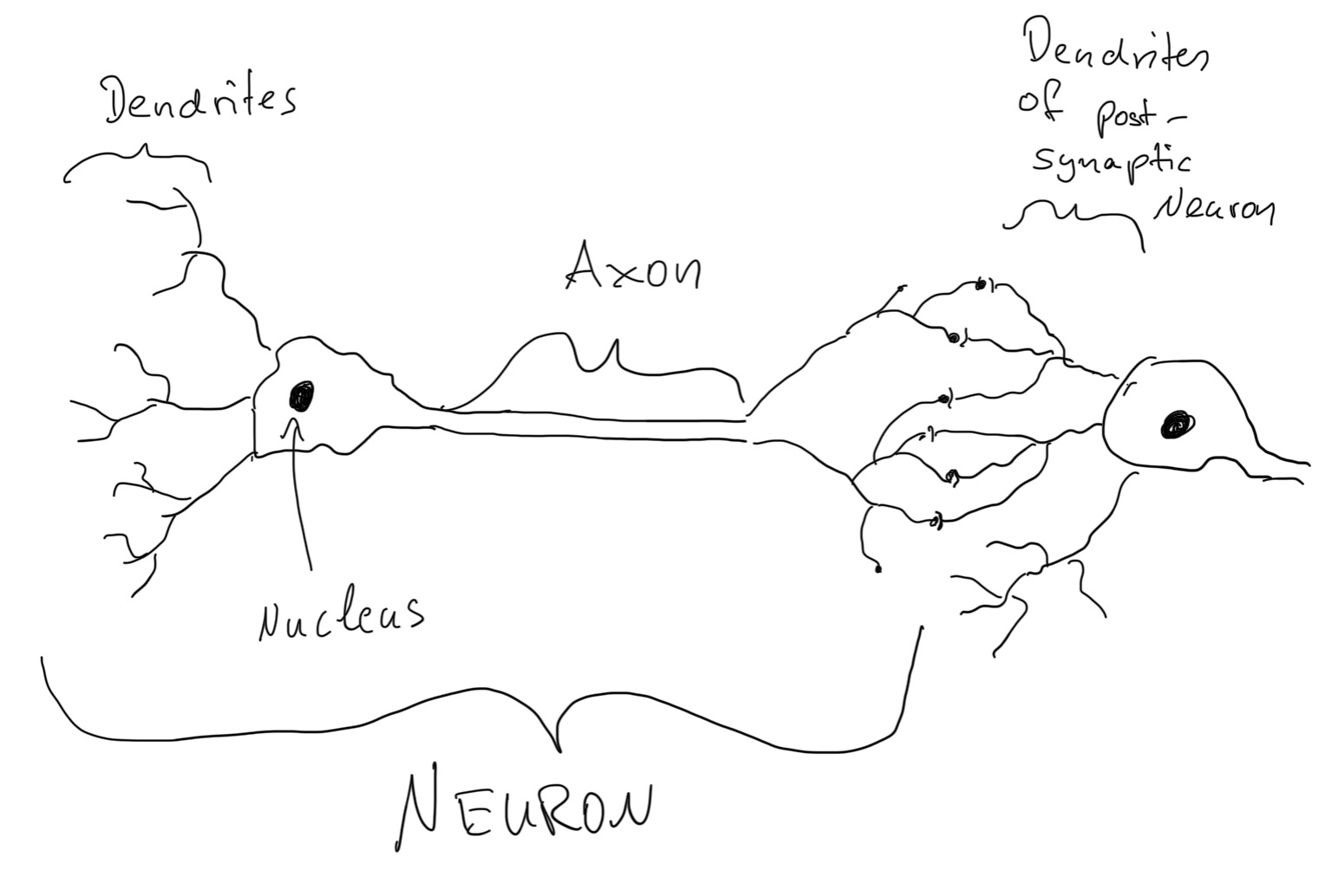
The perceptron is the most basic unit of neural networks. However, even for perceptron, there are so many different variants. In today’s lecture, our “Perceptron” will specifically represent “a classic Rosenblatt Perceptron”. This basically means we’ll use the threshold function as our activation function.
While we’ll be somewhat loose about the terminology here, we are building foundations that will lead us to multi-layer perceptrons (MLPs).
Terminology
Before everything starts, we need to declare our terminology used here.
Generally, like when we talk about logistic regression, multilayer nets and extra, our terminology follow the convention below:
- Net input = pre-activation = weighted input, $z$
- Activations = activation function (net input); $\alpha = \sigma(z)$
- Label output = threshold (activations of last layer); $\hat{y} = f(\alpha)$
For some speical cases, we may use some specifical terminology:
- In perceptron (the classic Rosenblatt Perceptron): activation function = threshold function
- In linear regression: activation = identity function ($f(x)=x$), so net input = output
Mathematical Formulation
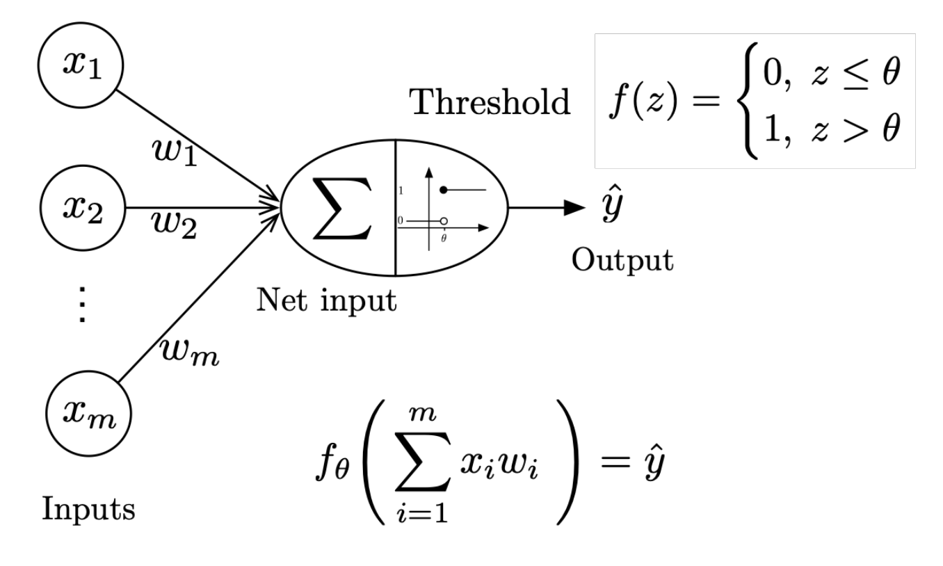
A perceptron takes multiple inputs $x_1, x_2, \ldots, x_n$ and produces a single binary output. The mathematical formulation is:
where:
- $w_i$ are the weights
- $b$ is the bias term
- $\sigma$ is the activation function (typically a step function for classical perceptrons)
Activation Functions
The activation function $\sigma$ determines the output of the perceptron. For the classical perceptron, we use a step function:
Handling Bias
In the above, the bias and the weights are seperate, this is not very convenient when we are actually doing the calculation. A common approach to deal with the bias in neural networks is to include the bias directly into the input vector $X$ by adding an extra dimension with a constant value of 1:
This allows us to write the perceptron output simply as:
More about the Activation Functions
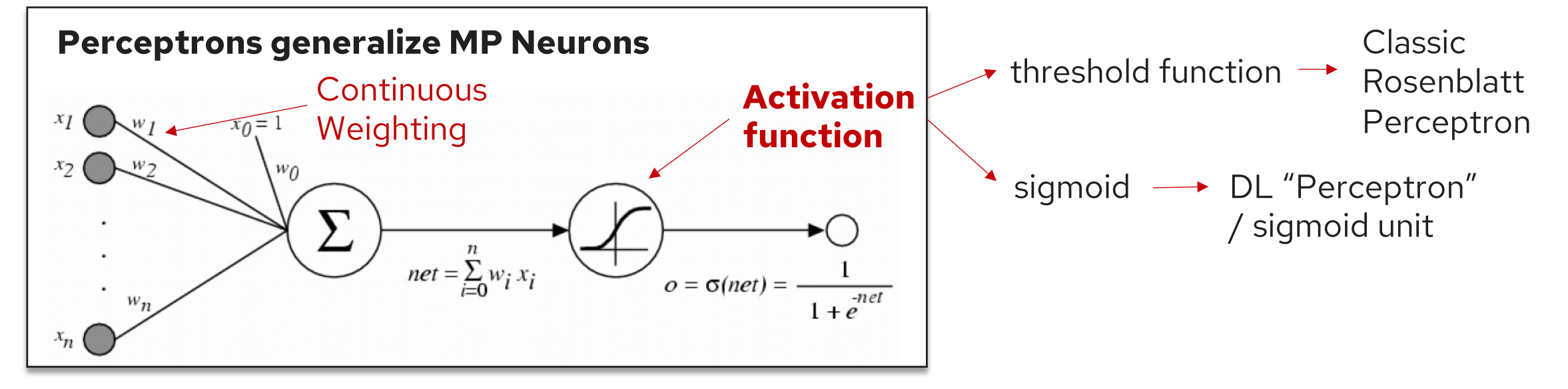
While the classical Rosenblatt perceptron uses the threshold function, modern neural networks employ various activation functions depending on the application and historical period:
Threshold Function (Perceptron, 1950+)
This is the original activation function used in Rosenblatt’s perceptron. It produces binary outputs but is not differentiable, making it unsuitable for gradient-based learning.
Sigmoid Function (before 2000)
The sigmoid function was widely used before 2000s. It’s smooth and differentiable, which enables backpropagation learning. However, it suffers from vanishing gradient problems in deep networks.
ReLU Function (popular since CNNs)
ReLU (Rectified Linear Unit) became popular with the rise of CNNs and deep learning. It’s computationally efficient and helps mitigate vanishing gradient problems.
Many Variants of ReLU
Modern deep learning employs numerous ReLU variants:
- Leaky ReLU: $\text{LeakyReLU}(z) = \max(\alpha z, z)$ where $\alpha$ is a small positive constant
- GeLU: $\text{GeLU}(z) = z \cdot \Phi(z)$ where $\Phi$ is the standard Gaussian CDF
- Swish: $\text{Swish}(z) = z \cdot \sigma(z)$
- Mish: $\text{Mish}(z) = z \cdot \tanh(\text{softplus}(z))$
Each variant addresses specific issues like dead neurons (Leaky ReLU) or provides smoother approximations to ReLU (GeLU, Swish).
Perceptron Learning Algorithm
The perceptron learning algorithm is a simple and elegant method for training a perceptron to classify linearly separable data. Here’s the formal algorithm:
Algorithm (Pseudocode)
Let the training dataset be:
Algorithm Steps:
-
Initialize $\mathbf{w} := \mathbf{0}^m$ (assume weight includes bias)
-
For every training epoch:
- For every $(\mathbf{x}^{[i]}, y^{[i]}) \in D$:
- $\hat{y}^{[i]} := \sigma(\mathbf{x}^{[i]T} \mathbf{w})$ ← Only 0 or 1
- $err := (y^{[i]} - \hat{y}^{[i]})$ ← Only -1, 0, or 1
- $\mathbf{w} := \mathbf{w} + err \times \mathbf{x}^{[i]}$
- For every $(\mathbf{x}^{[i]}, y^{[i]}) \in D$:
Algorithm (Detailed Logic)
The learning rule can be broken down into three cases:
- If correct: Do nothing
- When $\hat{y}^{[i]} = y^{[i]}$, then $err = 0$, so $\mathbf{w}$ remains unchanged
- If incorrect:
- If output is 0 (target is 1): Add input vector to weight vector
- $err = 1 - 0 = 1$, so $\mathbf{w} := \mathbf{w} + \mathbf{x}^{[i]}$
- If output is 1 (target is 0): Subtract input vector from weight vector
- $err = 0 - 1 = -1$, so $\mathbf{w} := \mathbf{w} - \mathbf{x}^{[i]}$
- If output is 0 (target is 1): Add input vector to weight vector
2. Geometric Intuition
It might seem weird at first why we can directly add or subtract weights during learning. The key insight is that for linear classifiers like perceptrons:
- Angle is important, scale isn’t: The decision boundary depends on the direction of the weight vector, not its magnitude
- This is why we can directly subtract weights during learning - we’re essentially rotating the decision boundary
Decision Boundaries
A perceptron creates a linear decision boundary in the input space. For a 2D input space with features $x_1$ and $x_2$, the decision boundary is defined by:
This is a straight line that separates the input space into two regions:
- Points where $w_1 x_1 + w_2 x_2 + b > 0$ are classified as class 1
- Points where $w_1 x_1 + w_2 x_2 + b \leq 0$ are classified as class 0
Weight Vector Interpretation
The weight vector $\mathbf{w} = [w_1, w_2]^T$ is perpendicular to the decision boundary. The direction of $\mathbf{w}$ points toward the positive class, and its magnitude affects the “confidence” of the classification.
Updating Weight Vector
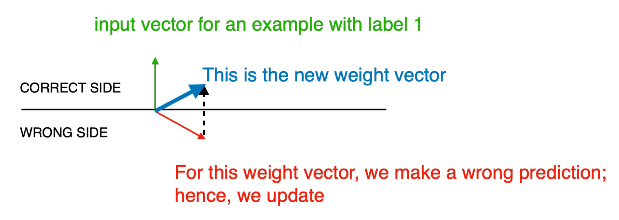
When a positive example x (green) is misclassified by the current weight vector w (red)—i.e.,
—we update the model by moving the weights toward the example:
Geometrically, this adds a step in the direction of x, rotating and shifting the decision boundary so that x moves to the correct side. The blue arrow shows the new weight vector after the update; the dashed line indicates the margin change.
Perceptron Limitations
- Linear only: Decision boundary is a hyperplane; no curved/non-linear splits.
- Binary output: One unit gives 0/1 only; multi-class needs extra machinery.
- Cannot solve XOR: XOR is not linearly separable → no single hyperplane fits.
- No convergence on non-separable data: If classes overlap/noisy, updates can oscillate.
- Many training optima, weak generalization: Many separating hyperplanes exist; the one found may have small margin and overfit.
Parallel Histories
- 1838 — Verhulst: introduces the logistic function (population growth).
- 1943 — McCulloch & Pitts: logic neurons (no learning).
- 1944 — Berkson: introduces the logit.
- 1957 — Rosenblatt: perceptron + learning rule (connectionism).
- 1958 — Cox: logistic regression as general regression (statistics).
- 1969 — Minsky & Papert: perceptron limits (can’t do XOR).
- 1986 — Rumelhart, Hinton & Williams: backpropagation + sigmoids.
- Can be seen as “solve the 1969 problem by stacking the 1958 model → MLE by gradient ascent / chain rule.”
Perceptrons and Deep Learning
- Core question: Why did the perceptron become the origin story for DL?
- Key reasons:
- A learning neuron: Rosenblatt framed a neuron with a simple learning rule and even built hardware—easy to rally around.
- Clear path to depth: Stack the same unit + backprop → multilayer networks; “logistic” sounds like a single-model family.
- Community + story: Connectionist culture popularized the “neurons that learn” narrative more than GLM language did.
- Historical timing: Perceptron arrived before modern stats/ML branding, so it became the origin tale by practice and momentum.
3. Notational Conventions for Neural Networks
Standard Notation
When working with neural networks, we typically use the following conventions:
- Input: $\mathbf{x} \in \mathbb{R}^d$ where $d$ is the input dimension
- Weights: $\mathbf{W} \in \mathbb{R}^{m \times d}$ for a layer with $m$ outputs and $d$ inputs
- Bias: $\mathbf{b} \in \mathbb{R}^m$
- Pre-activation: $\mathbf{z} = \mathbf{W}\mathbf{x} + \mathbf{b}$
- Activation: $\mathbf{a} = \sigma(\mathbf{z})$
A Fully-Connected Layer
With all the notation we have, we can come up with a fully-connected layer:
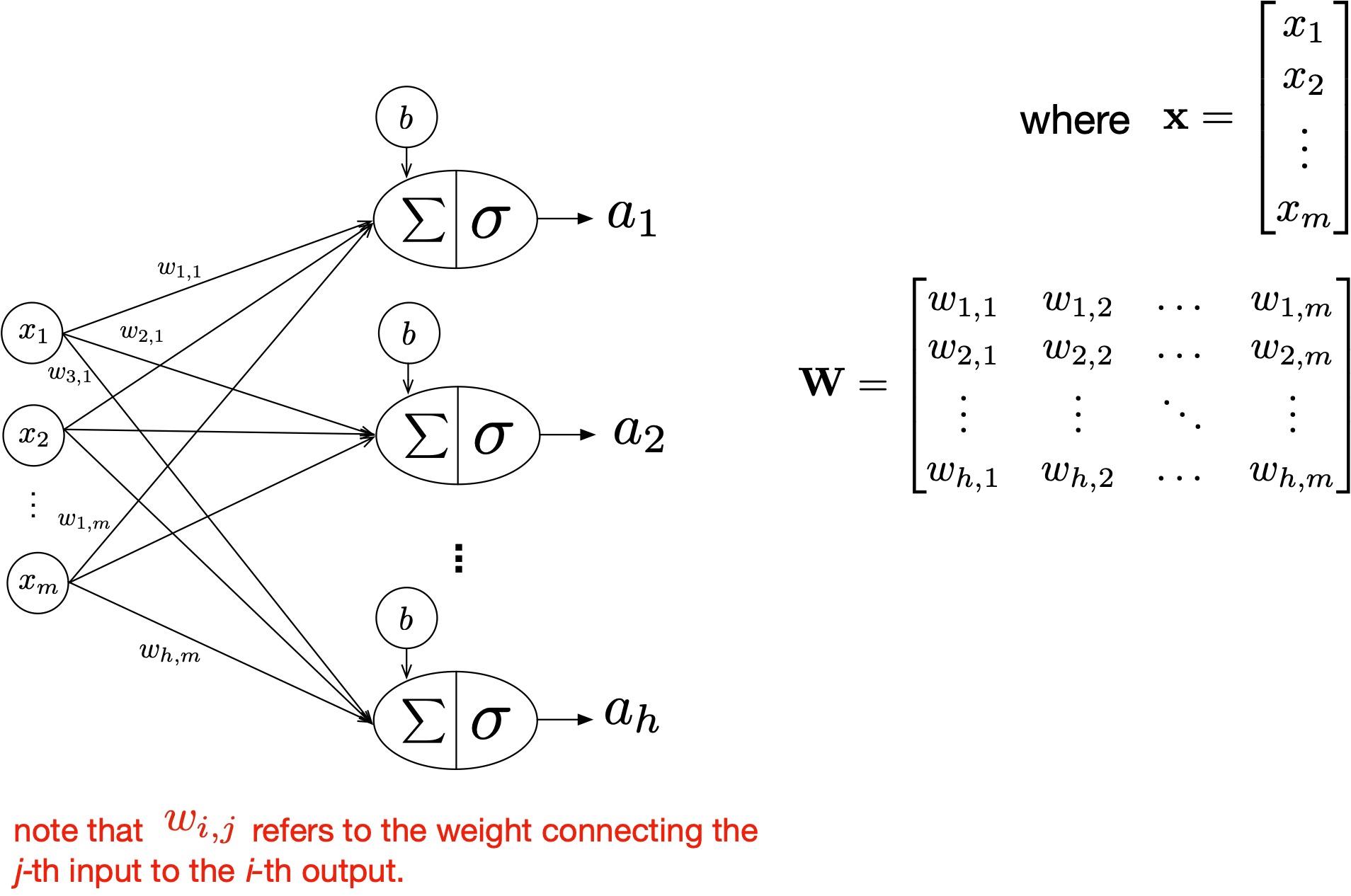
Matrix Form
For a batch of inputs $\mathbf{X} \in \mathbb{R}^{n \times d}$ (where $n$ is the batch size):
Intuition of W\mathbf{x} notation
- Column view: The output is a linear combination of the columns of (W) with weights (x) and (y).
- First column: (a) scales the (x)-coordinate; (c) moves (x) into the (y) direction.
- Second column: (b) moves (y) into the (x) direction; (d) scales the (y)-coordinate.
4. A Fully Connected (Linear) Layer in PyTorch
Implementation
In PyTorch, a fully connected layer is implemented using nn.Linear:
import torch
import torch.nn as nn

# Create a linear layer: input_size=784, output_size=10
linear_layer = nn.Linear(784, 10)

# Forward pass
x = torch.randn(32, 784)  # batch_size=32, input_size=784
output = linear_layer(x)  # output shape: (32, 10)
Understanding the Parameters
# Access weights and bias
print(f"Weight shape: {linear_layer.weight.shape}")  # (10, 784)
print(f"Bias shape: {linear_layer.bias.shape}")      # (10,)

# The operation performed is: output = x @ weight.T + bias
Building a Simple Perceptron
class Perceptron(nn.Module):
    def __init__(self, input_size):
        super(Perceptron, self).__init__()
        self.linear = nn.Linear(input_size, 1)
        self.activation = nn.Sigmoid()  # or nn.Heaviside for step function

    def forward(self, x):
        z = self.linear(x)
        return self.activation(z)

# Usage
perceptron = Perceptron(input_size=2)
x = torch.tensor([[1.0, 2.0], [3.0, 4.0]])
output = perceptron(x)
Key Takeaways
- Historical Significance: Rosenblatt’s perceptron laid the foundation for modern neural networks
- Linear Separation: Single-layer perceptrons can only solve linearly separable problems
- Geometric Interpretation: The weight vector defines the decision boundary orientation
- Mathematical Foundation: Understanding matrix operations is crucial for neural network implementation
- PyTorch Implementation:
nn.Linearprovides an efficient implementation of fully connected layers
Next Steps
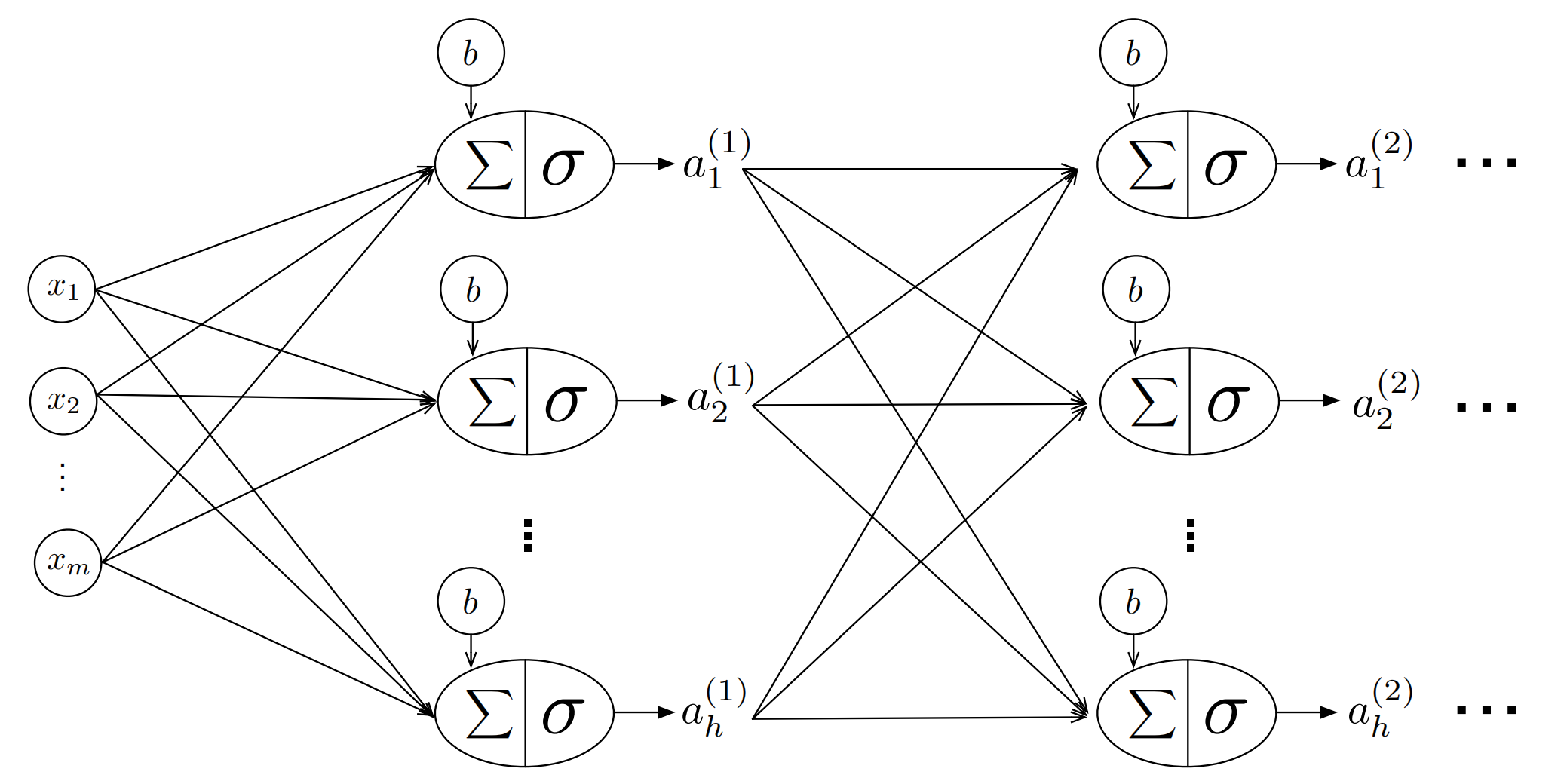
In the next lecture, we will explore:
- Multi-layer perceptrons (MLPs)
- How adding hidden layers enables non-linear decision boundaries
- The universal approximation theorem
- Backpropagation algorithm for training deep networks
Note: This lecture provides the fundamental building blocks that we’ll use throughout the course. Make sure you understand the geometric intuition and mathematical formulation before moving to more complex architectures. Only basic.