Lecture 05

Fitting Neurons with Gradient Descent

Lecture Overview

1. Online, batch, and minibatch mode
2. Relation between percetron and linear regression
3. An iterative training algorithm for linear regression
4. Calculus Refresher I: Derivatives
5. Calculus Refresher II: Gradients
6. Understanding gradient descent
7. Training an adaptive linear neuron (Adaline)

---

1. Online, batch, and minibatch mode

Perceptron Recap

, where

\sigma \!\Bigl( \sum_{i=1}^{m} x_i w_i + b \Bigr) = \sigma \!\bigl( \mathbf{x}^{T} \mathbf{w} + b \bigr) = \hat{y} \sigma(z) = \begin{cases} 0, & z \le 0 \\ 1, & z > 0 \end{cases} b = -\theta

---

Let $\mathcal{D} = (\langle \mathbf{x}^{[1]}, y^{[1]} \rangle, \mathbf{x}^{[2]}, y^{[2]} \rangle, \dots, \mathbf{x}^{[n]}, y^{[n]} \rangle) \in (\mathbb{R}^{m} \times {0,1})^{n} $.

1. Initialize $ \mathbf{w} := \mathbf{0} \in \mathbb{R}^{m}, \quad b := 0 $

2. For every training epoch:

   A. For every $ \langle x^{[i]}, y^{[i]} \rangle \in \mathcal{D} $:

   • (a) Compute output (prediction) $ \hat{y}^{[i]} := \sigma( x^{[i]\top} \mathbf{w} + b \bigr) $

   • (b) Calculate error $ \mathrm{err} := \bigl( y^{[i]} - \hat{y}^{[i]} \bigr) $

   • (c) Update parameters $ \mathbf{w} := \mathbf{w} + \mathrm{err} \times x^{[i]}, \quad b := b + \mathrm{err} $

“On-line” mode (= SGD: Schocastic Gradient Descent)

1. Initialize $ \mathbf{w} := \mathbf{0} \in \mathbb{R}^{m}, \quad b := 0 $

2. For every training epoch:

   A. For every $ \langle x^{[i]}, y^{[i]} \rangle \in \mathcal{D} $:

   • (a) Compute output (prediction)
   • (b) Calculate error
   • (c) Update $ \mathbf{w}, \mathbf{b}$

• For step 2, we usually shuffle the dataset prior to each epoch to prevent cycles
• Applies to all common neuron models and (deep) neural network architectures

“On-line” mode II (alternative)

1. Initialize $ \mathbf{w} := \mathbf{0} \in \mathbb{R}^{m}, \quad b := 0 $

2. For every training epoch:

   A. Pick random $ \langle x^{[i]}, y^{[i]} \rangle \in \mathcal{D} $:

   • (a) Compute output (prediction)
   • (b) Calculate error
   • (c) Update $ \mathbf{w}, \mathbf{b}$

• No shuffling required

Batch mode

1. Initialize $ \mathbf{w} := \mathbf{0} \in \mathbb{R}^{m}, \quad b := 0 $

2. For every training epoch:

   A. Take all training examples from $\mathcal{D} $:

   • (a) Compute output (prediction)
   • (b) Calculate error

   B. Update $ \mathbf{w}, \mathbf{b}$

Minibach mode (mix between on-line and batch)

1. Initialize $ \mathbf{w} := \mathbf{0} \in \mathbb{R}^{m}, \quad b := 0 $

2. For every training epoch:

   A. For every minibatch of size k, namely

   $ (\langle x^{[i]}, y^{[i]} \rangle, \dots, \langle x^{[i+k]}, y^{[i+k]} \rangle) \in \mathcal{D}$

   • (a) Compute output (prediction)
   • (b) Calculate error
   • (c) Update $ \mathbf{w} := \mathbf{w} + \Delta \mathbf{w}, \quad \mathbf{b} := \mathbf{b} + \Delta \mathbf{b} $

• This is the most common mode in deep learning because:
  1. choosing a subset instead of one example at a time takes advantage of vectorization (faster iteration through epoch than on-line)
  2. having fewer updates than “on-line” makes updates less noisy.
  3. makes more updates / epoch than “batch” and is thus faster

---

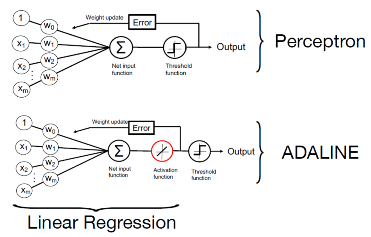
2. Relation between perceptron and linear regression

Perceptron

• activation function is the threshold function
• output is a binary label $\hat{y} \in ({0,1})$

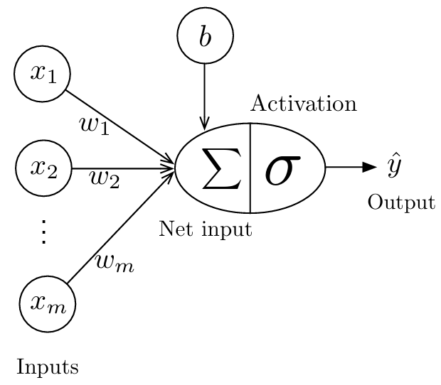
Linear Regression

• activation function is the identity function $ \sigma(x) = x $
• output is a real number $\hat{y} \in \mathbb{R}$
• you can think of linear regression as a linear neuron

(Least-Squares) Linear Regression

\mathbf{w} = (\mathbf{X}^{\top}\mathbf{X})^{-1}\mathbf{X}^{\top}y

, assuming the bias is included in $ \mathbf{w}$, and the design matrix has an additional vector of 1’s

• Generally, this is the best approach for linear regression

---

3. An iterative training algorithm for linear regression

(Least-Squares) Linear Regression

• A very naive way to fit a linear regression model (and any neural net) is to start with initializing the parameters to 0’s or small random values

• Then, for k rounds

  1. Choose another random set of weights
  2. If the model performs better, keep those weights
  3. If the model performs worse, discard the weights
• Guaranteed to find the optimal solution for very large k, but it would be terribly slow

Better way

• analyze what effect a change of a parameter has on the predictive performance (loss) of a model
• then change the weight a little in the direction that improves the performance (minimizes the loss) the most
• do this in several (small) steps until the loss does not further decrease

Update Rules (“on-line” mode)

Perceptron Learning Rule

1. Initialize $ \mathbf{w} := \mathbf{0} \in \mathbb{R}^{m}, \quad b := 0 $

2. For every training epoch:

   A. For every $ \langle x^{[i]}, y^{[i]} \rangle \in \mathcal{D} $:

   • (a) $ \hat{y}^{[i]} := \sigma\bigl(x^{[i]\top}\mathbf{w} + b\bigr) $
   • (b) $ err := \bigl(y^{[i]} - \hat{y}^{[i]}\bigr) $
   • (c) $ \mathbf{w} := \mathbf{w} + err \times x^{[i]}, \quad b := b + err $

Stochastic Gradient Descent (Vectorized)

1. Initialize $ \mathbf{w} := \mathbf{0} \in \mathbb{R}^{m}, \quad b := 0 $

2. For every training epoch:

   A. For every $ \langle x^{[i]}, y^{[i]} \rangle \in \mathcal{D} $:

   • (a) $ \hat{y}^{[i]} := \sigma\bigl(x^{[i]\top}\mathbf{w} + b\bigr) $

   • (b) $ \nabla_{\mathbf{w}}\mathcal{L} = \bigl(y^{[i]} - \hat{y}^{[i]}\bigr)x^{[i]}, \quad \nabla_{b}\mathcal{L} = \bigl(y^{[i]} - \hat{y}^{[i]}\bigr) $

   • (c) $ \mathbf{w} := \mathbf{w} + \eta \times \bigl(-\nabla_{\mathbf{w}}\mathcal{L}\bigr), \quad b := b + \eta \times \bigl(-\nabla_{b}\mathcal{L}\bigr) $

   where $\eta$ = learning rate, $\bigl(-\nabla_{\mathbf{w}}\mathcal{L}\bigr)$ = negative gradient

Stochastic Gradient Descent (For understanding only)

1. Initialize $ \mathbf{w} := \mathbf{0} \in \mathbb{R}^{m}, \quad b := 0 $

2. For every training epoch:

   A. For every $ \langle x^{[i]}, y^{[i]} \rangle \in \mathcal{D} $:

   • (a) $ \hat{y}^{[i]} := \sigma\bigl(x^{[i]\top}\mathbf{w} + b\bigr) $

   B. For weight $ \boldsymbol{j \in {1, \ldots, m}} $:

   • (b) $ \frac{\partial \mathcal{L}}{\partial w_{j}} = \bigl(y^{[i]} - \hat{y}^{[i]}\bigr)x_{j}^{[i]} $

   • (c) $ w_{j} := w_{j} + \eta \times \Bigl(-\frac{\partial \mathcal{L}}{\partial w_{j}}\Bigr) $

   C. $ \frac{\partial \mathcal{L}}{\partial b} = \bigl(y^{[i]} - \hat{y}^{[i]}\bigr) $, $ b := b + \eta \times \Bigl(-\frac{\partial \mathcal{L}}{\partial b}\Bigr) $

   where $\eta \times \Bigl(-\frac{\partial \mathcal{L}}{\partial b}\Bigr)$ coincidentally appears almost to be the same as the perceptron rule, except that the prediction is a real number, and we have a learning rate

This learning rule is called Gradient Descent

---

4. Calculus Refresher I: Derivatives

Differential Calculus Refresher

1. The derivative of a function $f(x)$ at a point $x=a$ is defined as the limit of the difference quotient (if it exists):

f'(a) = \lim\limits_{\Delta x \to 0} \frac{f(a+\Delta x) - f(a)}{\Delta x}

• $\Delta x$ represents an increment in x

1. If a function $f(x)$ is differentiable at every point of an interval A, we say that $f(x)$ is differentiable on A. In this case, for each $ x=a \in A$ there exists a derivative $f’(a)$ corresponding to it.

• This defines a new function on $A$, namely the derivative function $ f’(x)$

f'(x) = \frac{df}{dx} = \lim\limits_{\Delta x \to 0} \frac{f(x+ \Delta x) - f(x)}{ \Delta x}

• Examples

• $ f(x)=2x$:

f'(x)= \lim\limits_{\Delta x \to 0} \frac{f(x+\Delta x) - f(x)}{\Delta x}=\lim\limits_{\Delta x \to 0} \frac{2x+2\Delta x-2x}{\Delta x} =\lim\limits_{\Delta x \to 0} \frac{2\Delta x}{\Delta x}=2

• $ f(x)=x^2$:

f'(x)= \lim\limits_{\Delta x \to 0} \frac{f(x+\Delta x) - f(x)}{\Delta x}=\lim\limits_{\Delta x \to 0} \frac{x^2+2x \Delta x+(\Delta x)^2-x^2}{\Delta x} =\lim\limits_{\Delta x \to 0} \frac{2x \Delta x+(\Delta x)^2}{\Delta x}=\lim\limits_{\Delta x \to 0}2x+ \Delta x=2x

Cheatsheet 1: Frequently used derivative formulas

f(x) = a \quad \Rightarrow \quad f'(x) = 0 f(x) = x \quad \Rightarrow \quad f'(x) = 1 f(x) = ax \quad \Rightarrow \quad f'(x) = a f(x) = x^a \quad \Rightarrow \quad f'(x) = ax^{a-1} f(x) = a^x \quad \Rightarrow \quad f'(x) = \log(a) a^x f(x) = \log(x) \quad \Rightarrow \quad f'(x) = \frac{1}{x} f(x) = \log_a(x) \quad \Rightarrow \quad f'(x) = \frac{1}{x \log(a)} f(x) = \sin(x) \quad \Rightarrow \quad f'(x) = \cos(x) f(x) = \cos(x) \quad \Rightarrow \quad f'(x) = -\sin(x) f(x) = \tan(x) \quad \Rightarrow \quad f'(x) = \sec^2(x)

Cheatsheet 2: Derivative Rules

• Sum Rule

h(x) = f(x) + g(x), \quad h'(x) = f'(x) + g'(x)

• Difference Rule

h(x) = f(x) - g(x), \quad h'(x) = f'(x) - g'(x)

• Product Rule

h(x) = f(x) g(x), \quad h'(x) = f'(x) g(x) + f(x) g'(x)

• Quotient Rule

h(x) = \frac{f(x)}{g(x)}, \quad h'(x) = \frac{f'(x) g(x) - f(x) g'(x)}{g(x)^2}

• Reciprocal Rule

h(x) = \frac{1}{f(x)}, \quad h'(x) = \frac{-f'(x)}{f(x)^2}

• Chain Rule

h(x) = f(g(x)), \quad h'(x) = f'(g(x)) g'(x)

• The chain rule is the essence of training neural networks.

Chain Rule & Computation Graph

• For a nested function $ F(x)=f(g(x))=z$
• Its computational graph:

x \xrightarrow{g} g(x) \xrightarrow{f} f(g(x))=z

• Derivative of the nested function: $F’(x)=f’(g(x))g’(x)=z’$
• Computational graph of derivative function:

x \xrightarrow{g} g(x) \xrightarrow{f'} f'(g(x)) x \xrightarrow{g'} g'(x) f'(g(x)) \cdot g'(x)=z'

• Pytorch keeps computational graphs in the background and computes the derivatives of most differentiable functions automatically.

Chain Rule & Leibniz Notation

• For efficiency, we use the Leibniz notation:

\frac{d}{dx}[f(g(x))]=\frac{df}{dg}\cdot \frac{dg}{dx}

• this is useful when writing long function compositions:

\frac{d}{dx}[f(g(h(u(v(x)))))]=\frac{df}{dg}\cdot \frac{dg}{dh} \cdot \frac{dh}{du} \cdot \frac{du}{dv} \cdot \frac{dv}{dx}

• Here’s an example of implementing the Chain Rule (using Leibniz notation):

• $f(x)=\log(\sqrt{x})$:

\frac{d}{dg}\log(g)=\frac{1}{g}=\frac{1}{\sqrt{x}} \frac{d}{dx}x^{\frac{1}{2}}=\frac{1}{2 \sqrt{x}} \frac{df}{dx}=\frac{1}{2 \sqrt{x}}\cdot\frac{1}{\sqrt{x}}=\frac{1}{2x}

• reverse mode and forward mode:
• notice that:

\frac{df}{dg}\cdot \frac{dg}{dh} \cdot \frac{dh}{du} \cdot \frac{du}{dv} \cdot \frac{dv}{dx} (reverse\ mode\: start\ from\ the\ outer\ parts ) = \frac{dv}{dx} \cdot \frac{du}{dv} \cdot \frac{dh}{du} \cdot \frac{dg}{dh} \cdot \frac{df}{dg}(forward\ mode\: start\ from\ the\ inner\ parts)

• Backpropagation is basically “reverse mode” auto-differentiation. It is cheaper than forward mode if we work with gradients because we would have matrix-vector multiplications instead of matrix-matrix multiplications.

5. Calculus Refresher II: Gradients

Derivatives of Multivariable Functions

1. For a multivariable function $f(x_1,x_2,x_3,…x_m)$:

\nabla f(\mathbf{\vec{x}}) = \begin{bmatrix} \frac{\partial f}{\partial x_1} \\ \frac{\partial f}{\partial x_2} \\ \vdots \\ \frac{\partial f}{\partial x_m} \end{bmatrix} \in \mathbb{R}^{m \times 1}

• Example:
• $f(x,y)=x^2y+y$

\nabla f(\mathbf{x,y}) = \begin{bmatrix} \frac{\partial f}{\partial x} \\ \frac{\partial f}{\partial y} \\ \end{bmatrix}= \begin{bmatrix} 2xy \\ x^2+1 \\ \end{bmatrix}

Multivariable Chain Rule

\frac{d}{dx}[f(g(x),h(x))]=\frac{\partial f}{\partial g} \cdot \frac{\partial g}{\partial x}+ \frac{\partial f}{\partial h} \cdot \frac{\partial h}{\partial x}

• Example:
  • $f(g,h)=g^2h+h$, where $g(x)=3x$ and $h(x)=x^2$

\frac{d}{dx}[f(g(x),h(x))]= 2gh \cdot 3+(g^2+1)\cdot 2x = 2xg^2+6gh+2x

Multivariable Chain Rule in vector form

\frac{\partial f}{\partial x} = \begin{bmatrix} \frac{\partial f}{\partial g} & \frac{\partial f}{\partial h} \end{bmatrix} \begin{bmatrix} \frac{\partial g}{\partial x} \\ \frac{\partial h}{\partial x} \end{bmatrix}= \frac{\partial f}{\partial g} \frac{\partial g}{\partial x} + \frac{\partial f}{\partial h} \frac{\partial h}{\partial x}

• define:

\mathbf{v}(x) = \begin{bmatrix} g(x) \\ h(x) \end{bmatrix}

• and:

\mathbf{v'}(x) = \begin{bmatrix} \frac{dg}{dx} \\ \frac{dh}{dx} \end{bmatrix}

• we also have:

\nabla f(\mathbf{g,h})= \begin{bmatrix} \frac{\partial f}{\partial g} \\ \frac{\partial f}{\partial h} \end{bmatrix}

• Putting it together:

\frac{\partial f}{\partial x}= \nabla f(\mathbf{g,h}) \cdot \mathbf{v}'(x) = \begin{bmatrix} \frac{\partial f}{\partial g} & \frac{\partial f}{\partial h} \end{bmatrix} \begin{bmatrix} \frac{dg}{dx} \\ \frac{dh}{dx} \end{bmatrix}= \frac{\partial f}{\partial g} \frac{dg}{dx} + \frac{\partial f}{\partial h} \frac{dh}{dx}

The Jacobian Matrix

\mathbf{f}(\mathbf{x}) = \begin{bmatrix} f_1(x_1, x_2, \dots, x_m) \\ f_2(x_1, x_2, \dots, x_m) \\ \vdots \\ f_m(x_1, x_2, \dots, x_m) \end{bmatrix}, \quad J(\mathbf{x}) = \frac{\partial \mathbf{f}}{\partial \mathbf{x}} = \begin{bmatrix} \frac{\partial f_1}{\partial x_1} & \frac{\partial f_1}{\partial x_2} & \cdots & \frac{\partial f_1}{\partial x_m} \\ \frac{\partial f_2}{\partial x_1} & \frac{\partial f_2}{\partial x_2} & \cdots & \frac{\partial f_2}{\partial x_m} \\ \vdots & \vdots & \ddots & \vdots \\ \frac{\partial f_m}{\partial x_1} & \frac{\partial f_m}{\partial x_2} & \cdots & \frac{\partial f_m}{\partial x_m} \end{bmatrix} \in \mathbb{R}^{m \times m}

• The i-th row of the Jacobian matrix is the gradient vector of $f_i$:

\nabla f_i(\mathbf{x}) = \begin{bmatrix} \frac{\partial f_i}{\partial x_1} \\ \frac{\partial f_i}{\partial x_2} \\ \vdots \\ \frac{\partial f_i}{\partial x_m} \end{bmatrix} \in \mathbb{R}^{m \times 1}

6. Understanding Gradient Descent

Back to Linear Regression

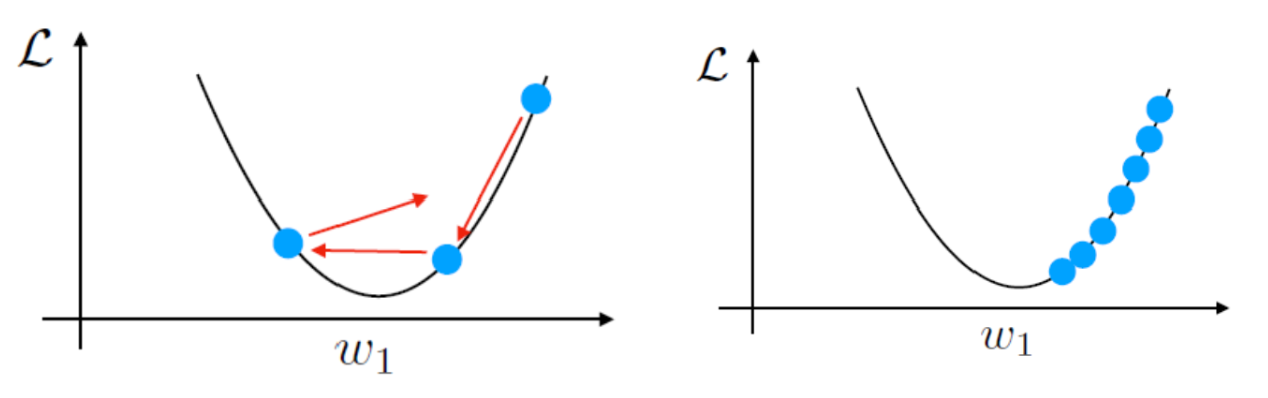
Gradient Descent

• Learning rate and steepness of the gradient determine how much we update
• Steps get smaller as you get toward the minimum
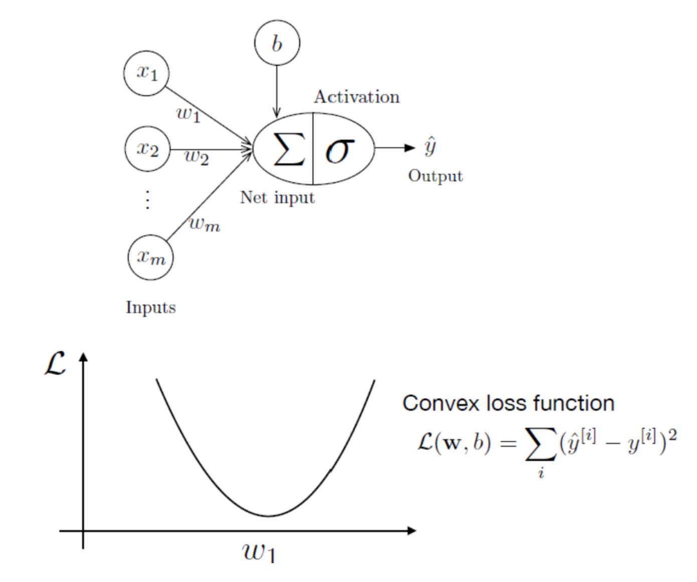
• Squared error gives convex loss function
• MSE loss is convex loss because we assume it’s the Sum Squared Error (SSE) or Mean Squared Error (MSE)

\text{SSE}(y, \hat{y}) = \sum_i (y_i - \hat{y}_i)^2

• Not every loss is convex
• Start with large learning rates and get smaller over time

Benefits of convexity:

• Especially for linear models, it is often not possible to achieve a zero loss even on the training data.
• Theoretical guarantee of convexity: reaching a unique minimizer efficiently.
• For general neural networks (due to nonlinear activation), no guarantee.
• If the learning rate is too large, we can overshoot, and if the learning rate is too small, convergence is very slow.

---

Returning to Previous Notes on Least-Squares Linear Regression

The update rule turns out to be this:

“On-line” mode (Perceptron learning rule)

1. Initialize

\mathbf{w} := 0 \in \mathbb{R}^m, \quad b := 0

1. For every training epoch:
   • For every $\langle x^{[i]}, y^{[i]} \rangle \in D$

\hat{y}^{[i]} := x^{[i]\top} \mathbf{w} + b \text{err} := y^{[i]} - \hat{y}^{[i]} \mathbf{w} := \mathbf{w} + \text{err} \cdot x^{[i]}, \quad b := b + \text{err}

Stochastic Gradient Descent (SGD)

1. Initialize

\mathbf{w} := 0, \quad b := 0

1. For every training epoch:
   • For every $\langle x^{[i]}, y^{[i]} \rangle \in D$

\hat{y}^{[i]} := x^{[i]\top} \mathbf{w} + b \mathbf{w} := \mathbf{w} - \eta \cdot \nabla_\mathbf{w} L, \quad b := b - \eta \cdot \nabla_b L

• Where eta is the learning rate .

---

Linear Regression Loss Derivative

Sum of Squared Error (SSE) loss is also called squared loss.

\mathcal{L}(\mathbf{w}, b) = \sum_i \bigl(\hat{y}^{[i]} - y^{[i]}\bigr)^2 \frac{\partial \mathcal{L}}{\partial w_j} = \frac{\partial}{\partial w_j} \sum_i \bigl(\hat{y}^{[i]} - y^{[i]}\bigr)^2 = \frac{\partial}{\partial w_j} \sum_i \bigl(\sigma(\mathbf{w}^\top x^{[i]}) - y^{[i]}\bigr)^2 = \sum_i 2\bigl(\sigma(\mathbf{w}^\top x^{[i]}) - y^{[i]}\bigr) \frac{\partial}{\partial w_j}\bigl(\sigma(\mathbf{w}^\top x^{[i]}) - y^{[i]}\bigr) = \sum_i 2\bigl(\sigma(\mathbf{w}^\top x^{[i]}) - y^{[i]}\bigr) \frac{d\sigma}{d(\mathbf{w}^\top x^{[i]})} \frac{\partial}{\partial w_j}\mathbf{w}^\top x^{[i]} = \sum_i 2\bigl(\sigma(\mathbf{w}^\top x^{[i]}) - y^{[i]}\bigr) \frac{d\sigma}{d(\mathbf{w}^\top x^{[i]})} \, x_j^{[i]}

• These equations show SSE.
• The activation function is the identity function in linear regression.

---

Alternative Linear Regression Loss Derivative

Mean Squared Error (MSE) often scales by factor ½ for convenience.

\mathcal{L}(\mathbf{w}, b) = \frac{1}{2n} \sum_i \bigl(\hat{y}^{[i]} - y^{[i]}\bigr)^2 \frac{\partial \mathcal{L}}{\partial w_j} = \frac{\partial}{\partial w_j} \frac{1}{2n} \sum_i \bigl(\hat{y}^{[i]} - y^{[i]}\bigr)^2 = \frac{\partial}{\partial w_j} \sum_i \frac{1}{2n}\bigl(\sigma(\mathbf{w}^\top x^{[i]}) - y^{[i]}\bigr)^2 = \sum_i \frac{1}{n}\bigl(\sigma(\mathbf{w}^\top x^{[i]}) - y^{[i]}\bigr) \frac{\partial}{\partial w_j}\bigl(\sigma(\mathbf{w}^\top x^{[i]}) - y^{[i]}\bigr) = \frac{1}{n}\sum_i \bigl(\sigma(\mathbf{w}^\top x^{[i]}) - y^{[i]}\bigr) \frac{d\sigma}{d(\mathbf{w}^\top x^{[i]})} \frac{\partial}{\partial w_j}\mathbf{w}^\top x^{[i]} = \frac{1}{n}\sum_i \bigl(\sigma(\mathbf{w}^\top x^{[i]}) - y^{[i]}\bigr) \frac{d\sigma}{d(\mathbf{w}^\top x^{[i]})} \, x_j^{[i]}

• These equations show MSE.
• The activation function is the identity function in linear regression.

---

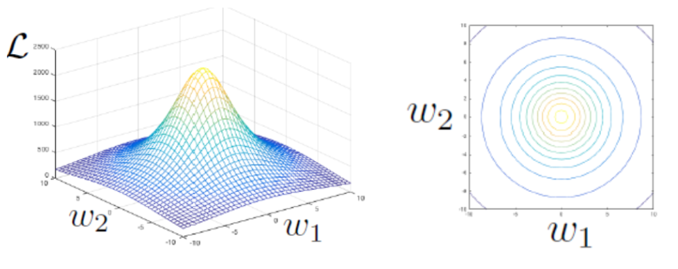
How to Think About Contour Plots

The following show the loss plot for two weights as a contour plot and flattened into a 2D space. As you can see, updates are perpendicular to contour lines.

---

Stochastic Gradient Descent as Surface Plot

Stochastic updates are a bit noisier because each minibatch is an approximation of the overall loss on the training set.

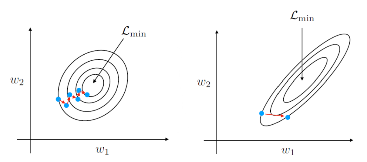
• These figures depict stochastic gradient descent.
• If inputs are on very different scales, some weights will update more than others which will also harm convergence. This is why we always normalize inputs.
• Stochastic (on-line or minibatch) are noisier than batch (whole-training-set) gradient descent.

Analogy:
Imagine you are a scientist who develops a new pharmaceutical drug.

• To know its average effectiveness, you’d test it on all patients in the world (like batch GD).
• This is expensive and slow.
• Instead, you select a smaller group of patients (like minibatch).
• Your estimate won’t be perfect, but if the sample is large enough, it’s accurate enough to guide improvements.

---

7. Training and Adaptive Linear Neuron (Adaline)

(Least-Squares) Linear Regression

We want to speed up computations and memory when input data has large dimensions.

\mathbf{w} = (\mathbf{X}^{\top}\mathbf{X})^{-1}\mathbf{X}^{\top}y

Assuming the bias is included in w, and the design matrix has an additional vector of 1’s.

---

ADALINE

Widrow and Hoff’s ADALINE (1960): A nicely differential neuron model.

• Stands for ADAptive LInear NEuron.