Lecture 09

Multilayer Perceptrons & Backpropagation

Today’s Topics:

Today’s Topics:
1. Multilayer Perceptron Architecture
2. Nonlinear Activation Functions
3. Multilayer Perceptron Code Examples
4. Overfitting and Underfitting (intro)

1. Multilayer Perceptron Architecture

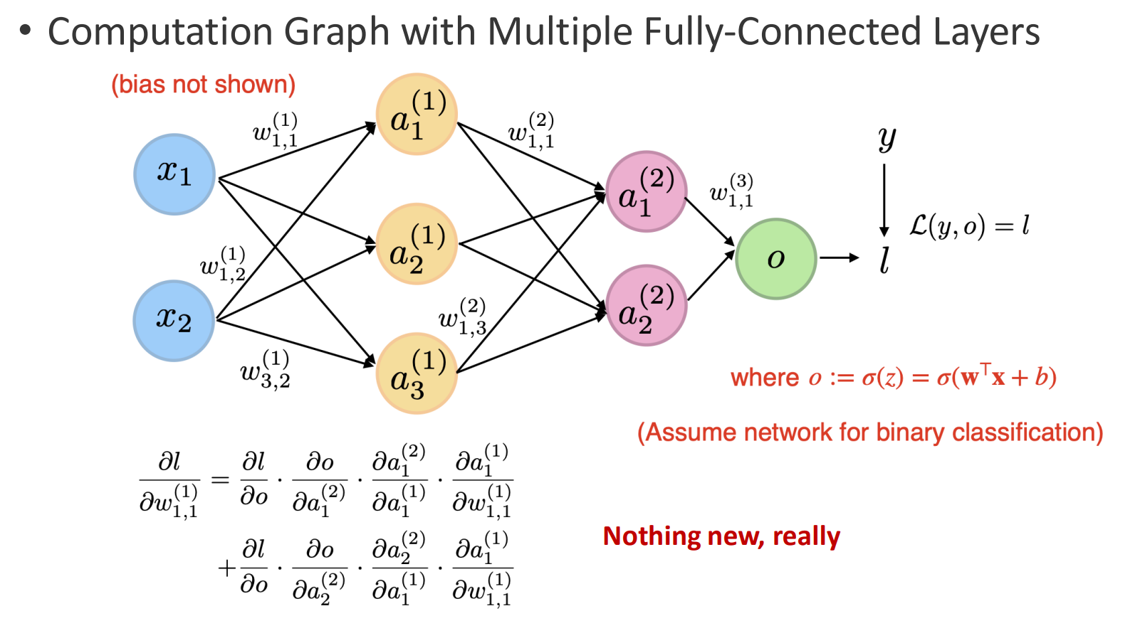
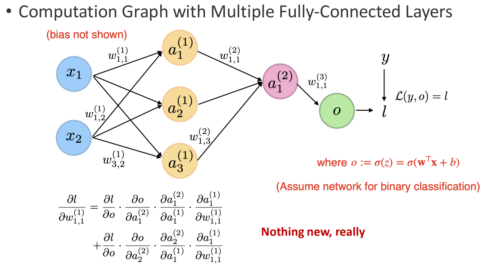
The Multilayer Perceptron (MLP) is a neural network model that extends the single-layer perceptron by stacking multiple fully connected layers into a computation graph. Each layer performs a linear transformation followed by a nonlinear activation function, enabling the network to capture non-linear relationships and hierarchical features.

Key Points:

Definition
- An MLP consists of multiple layers where each neuron in one layer connects to every neuron in the next.
- This structure generalizes linear models and enables more powerful function approximation than the basic perceptron, which can only output a single bit of information (0 or 1).
- Illustration:

2. Growth of Parameters (Slide 10)

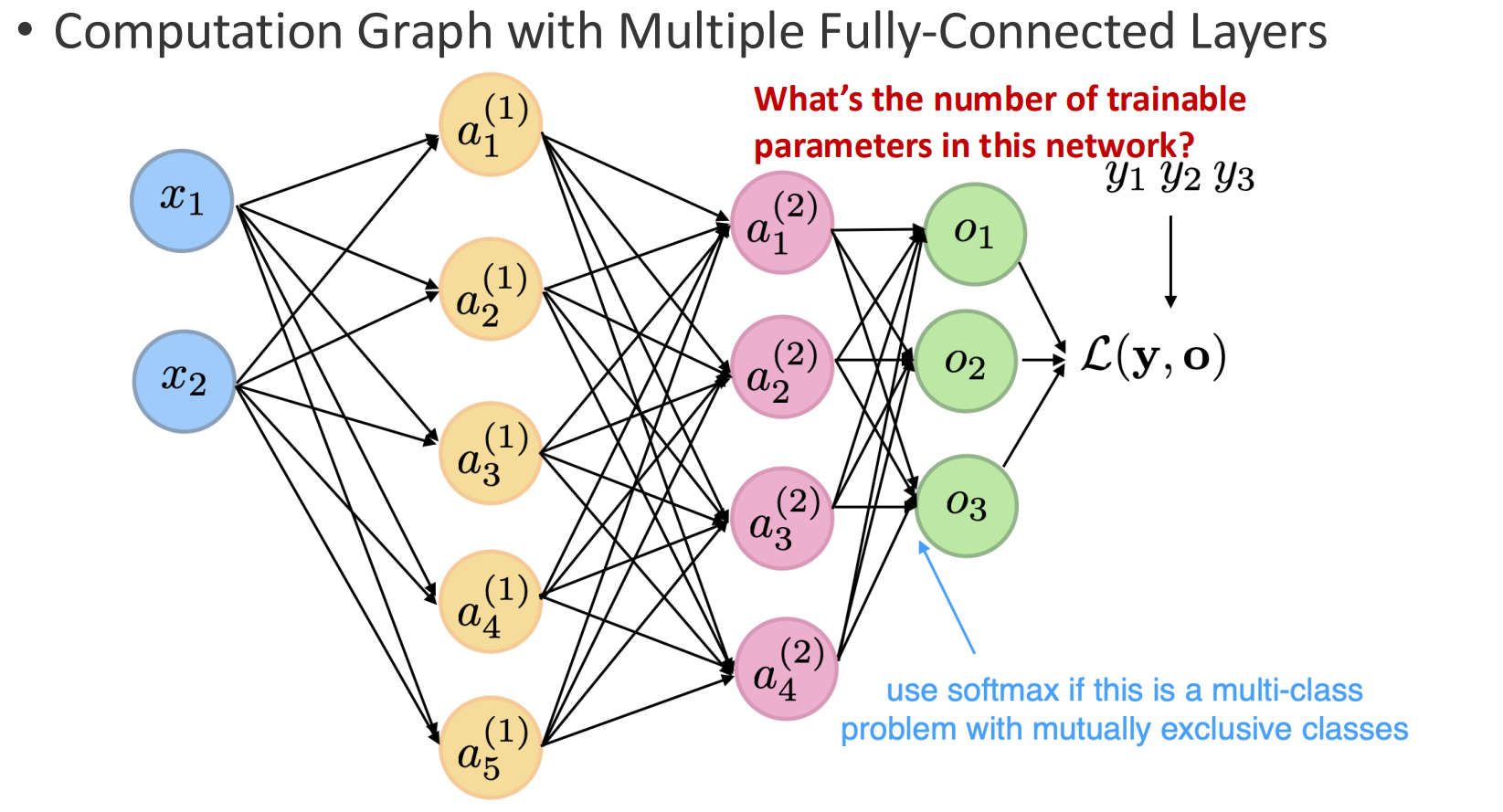
Every connection introduces a weight and a bias. As the network grows, the number of trainable parameters increases rapidly.
This highlights both the expressive power of MLPs and their tendency to overfit.

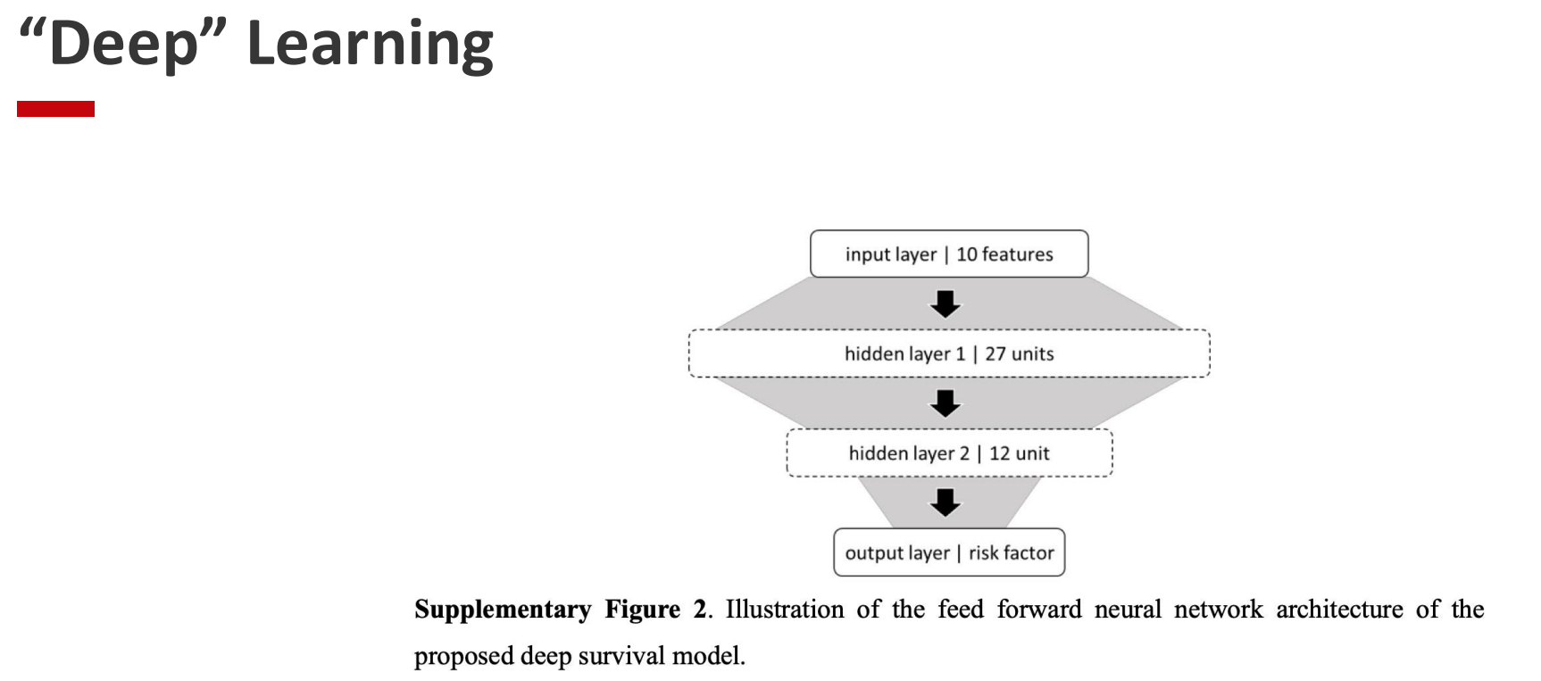
3. From “Shallow” to “Deep” (Slide 11)

Adding more layers leads to deep learning.

Shallow networks can already approximate many functions, but depth enables hierarchical feature learning.
Early layers capture simple features, while deeper layers build on them to represent complex structures.

This is the conceptual leap from “just a perceptron with more neurons” to the foundation of deep architectures.

4. Optimization Landscape: Convex vs. Non-convex (Slides 12–17)

Earlier models (e.g., logistic regression, adaline) had convex loss functions, ensuring one global minimum.
Formally, a function $f$ is convex if:

\[f(\lambda x + (1-\lambda)y) \leq \lambda f(x) + (1-\lambda) f(y), \quad \forall x,y,\; \lambda \in [0,1].\]

Convex optimization is simple: gradient descent always finds the global optimum.
MLPs instead have non-convex loss surfaces full of local minima and saddle points.
Training outcomes vary with initialization or data ordering, yet in practice many local minima perform equally well.
As Yann LeCun pointed out, non-convexity is not a dealbreaker — deep learning still succeeds despite it.

5. Importance of Initialization (Slide 18)

If all weights are initialized to zero, every neuron behaves identically, and the network cannot learn. The model would not be able to distinguish any importance of the nodes.
To break symmetry and ensure effective learning, random initialization (centered at zero, with variance scaled properly) and input normalization are essential.

Logical Flow

Start (Slides 5–6): Define what an MLP is — a layered computation graph.
Next (Slide 10): Show the cost of this design — many parameters to train.
Then (Slide 11): Extend the idea — depth brings hierarchical power.
Follow-up (Slides 12–17): Explain why optimization becomes harder (convex vs. non-convex).
Conclusion (Slide 18): Stress initialization — without it, even powerful architectures fail.

2. Nonlinear Activation Functions

Nonlinear activation functions are the key to making multilayer perceptrons more powerful than simple linear models. Without non-linearity, stacking multiple layers would still result in a single linear transformation, offering no advantage over logistic regression. By introducing nonlinear functions at each layer, MLPs can learn non-linear decision boundaries and solve problems like XOR that linear models fail to capture.

1. Why Nonlinearity Matters (Slide 21)

The XOR problem illustrates the limitation of linear classifiers: no single straight line can separate XOR’s outputs.
By applying nonlinear activations in hidden layers, MLPs can combine multiple linear boundaries into a nonlinear solution.
This is the central reason MLPs succeed where perceptrons fail.

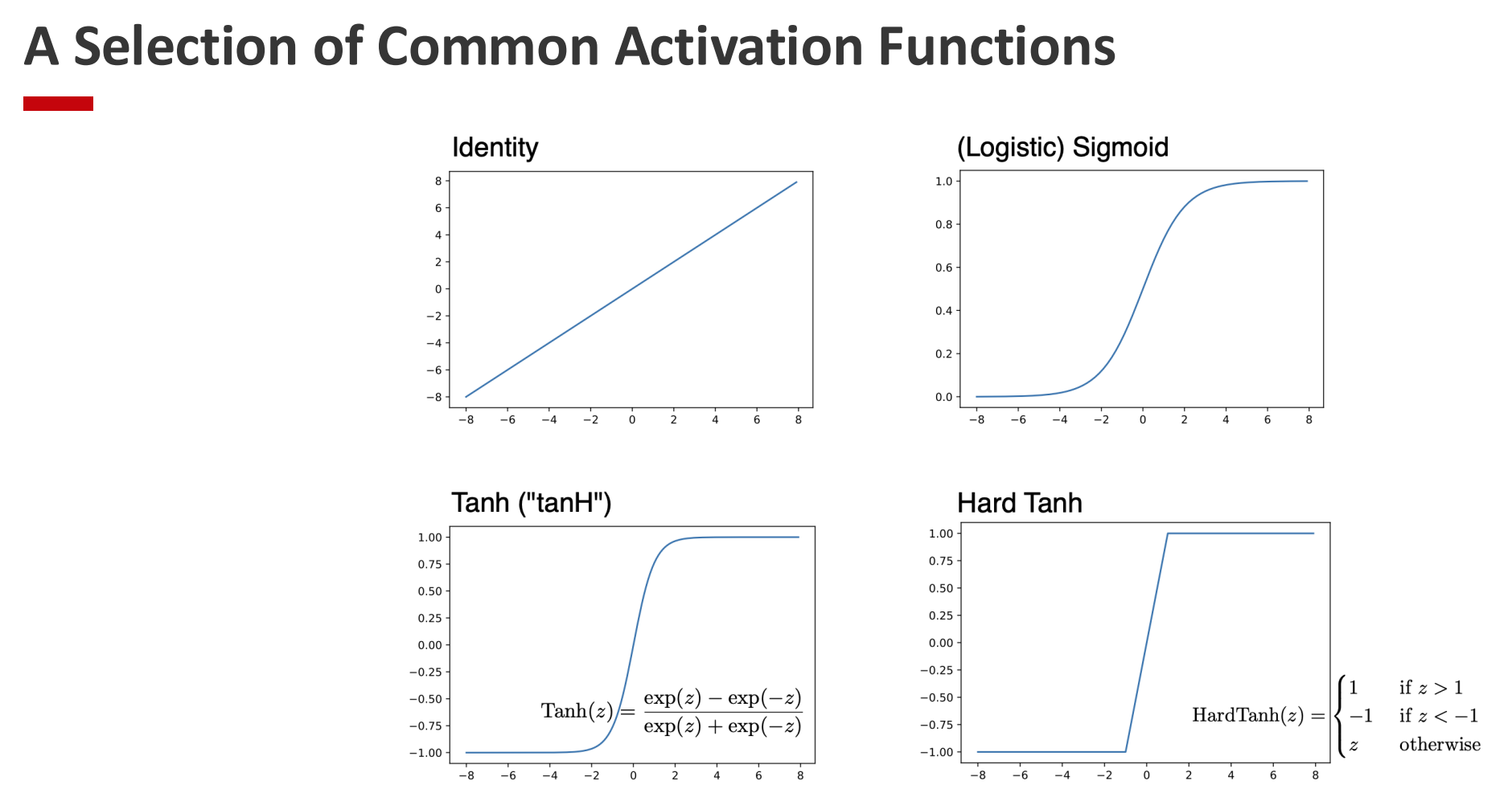
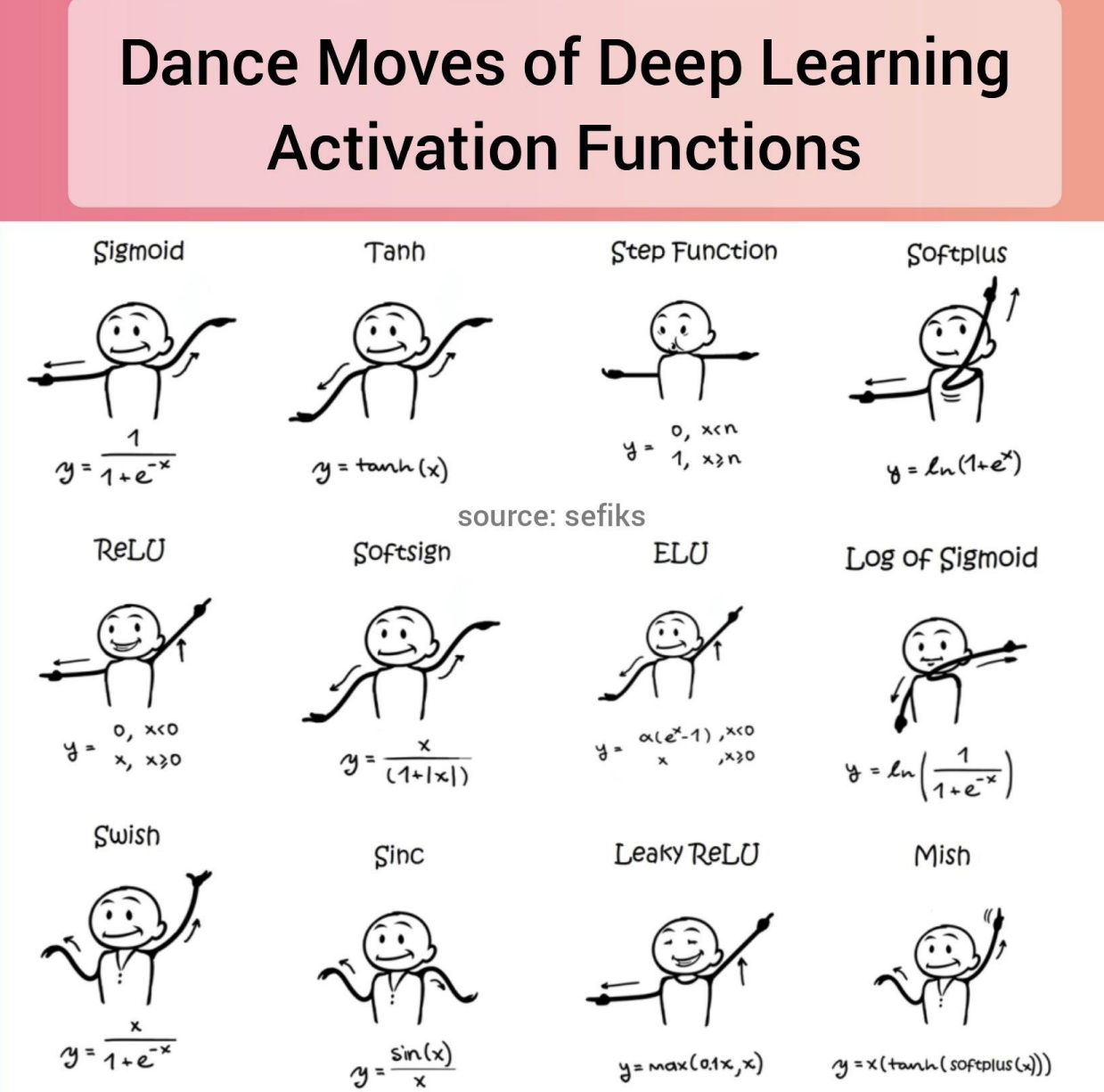
2. Common Activation Functions (Slides 22–24)

Several nonlinear activation functions are widely used. Each has its benefits and drawbacks:

Sigmoid: $ \sigma(x) = \frac{1}{1+e^{-x}} $
- Outputs between 0 and 1.
- Historically important, but suffers from vanishing gradients for large $ x $.
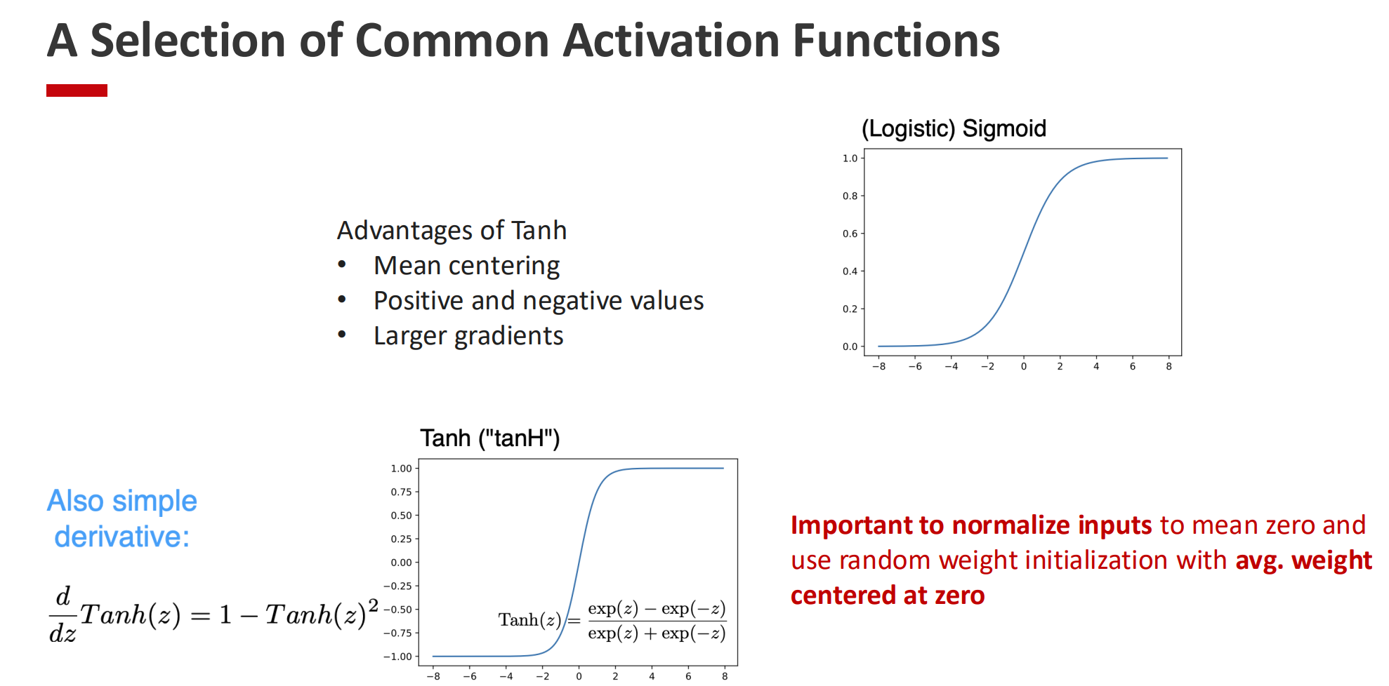
Tanh: $ \tanh(x) $
- Outputs between -1 and 1, centered around zero.
- Provides stronger gradients than sigmoid, but still saturates at extremes.
- Works best when inputs are normalized to zero mean.
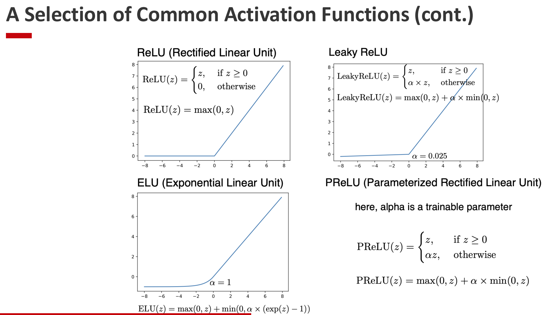
ReLU: $ \max(0, x) $
- Simple, fast to compute, avoids saturation for positive inputs.
- Risk of “dying ReLUs” (neurons stuck at zero).
Variants (Leaky ReLU, Smooth ReLU, etc.)
- Address ReLU’s shortcomings, e.g. keeping small gradients for negative inputs.

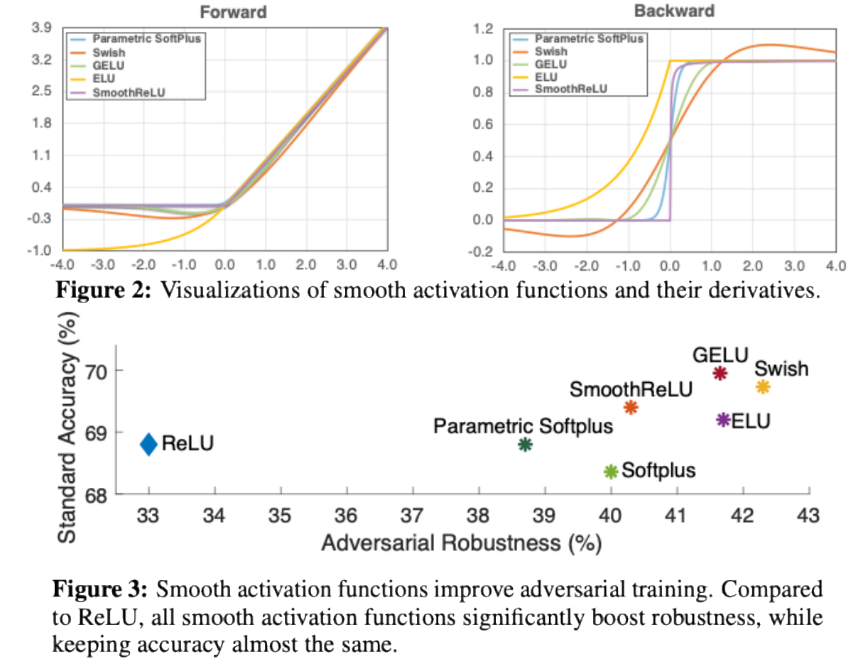
3. Activation Functions and Robustness (Slides 25–26)

Recent research shows that the choice of activation can influence not just accuracy, but also robustness.
For example, ReLU’s non-smooth nature can weaken adversarial training.
Replacing ReLU with smoother alternatives can improve both robustness and stability under adversarial attacks.

Logical Flow

Start (Slide 21): Motivate with XOR — why linear models fail.
Next (Slides 22–24): Present the main activation functions, with strengths and weaknesses.
Then (Slides 25–26): Highlight modern insights — activation choice also affects robustness, not just expressiveness.

Takeaway: Nonlinear activations unlock the true power of MLPs. They not only allow non-linear decision boundaries but also shape training dynamics, convergence, and robustness.

3. Multilayer Perceptron Code Examples

What to check before training

Set random seed for reproducibility (and log the random seed and package versions).
Check datasets and input data are as expected before training (shapes, dtypes, ranges, labels, NaNs).
Set timer, generator log, and print intermediate values to verify the training loop.
During training, if the loss behaves strangely (e.g., going up prematurely), stop and start diagnosis/debugging.
Change training hyperparameters and repeat experiments (learning rate, weight decay, batch size, scheduler, dropout).

Diagnosing Loss Curves

Compare training and validation/test loss to identify issues.
If validation loss plateaus or rises while training loss decreases, this often indicates overfitting → may require regularization or early stopping.
Training loss curves are often smoothed over mini-batches to reduce noise.
Some architectures (e.g., Transformers) show unusual training dynamics, such as sharp drops followed by long plateaus (“grokking”).
Loss curve behavior is strongly influenced by learning rate, LR scheduling, and initialization, so experimentation is often necessary.

4. Overfitting and Underfitting (intro)

Training vs. Generalization Error

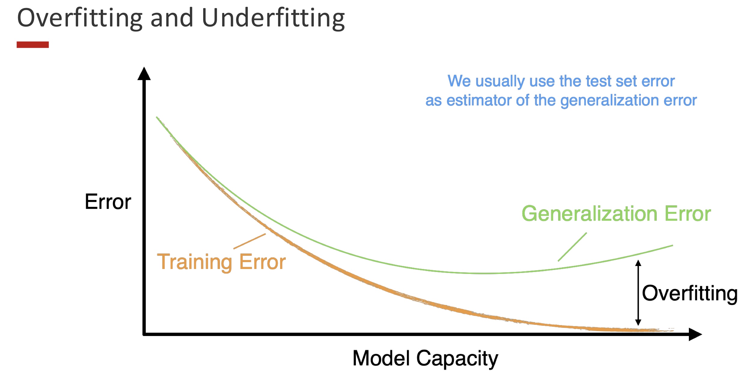
Big picture.

Training error (orange) typically decreases monotonically as model capacity increases.
Generalization (test/validation) error (green) first decreases (model fits signal better), then increases when the model starts to fit noise → overfitting.
The gap on the right is the classic sign of overfitting: low training loss, higher test loss.

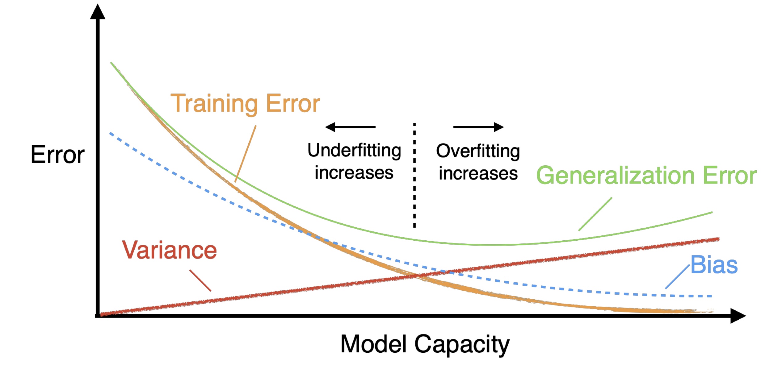
Bias–Variance Decomposition — Formulas

General definition

\[\mathrm{Bias}_\theta[\hat{\theta}] \=\ \mathbb{E}_\theta[\hat{\theta}] \-\ \theta\] \[\mathrm{Var}_\theta[\hat{\theta}] \=\ \mathbb{E}_\theta[\hat{\theta}^{2}] \-\ \big(\mathbb{E}_\theta[\hat{\theta}]\big)^{2}\]

Intuition

Why Deep Learning Loves Large Datasets

Traditional ML (blue, dashed): improves, then plateaus; limited capacity can’t keep exploiting more data.
Deep learning (green): with huge capacity, it keeps improving as dataset size grows—big data helps tame variance and lets the network learn richer invariances/features.
deep nets need lots of data to fully realize their capacity without overfitting.

Double Descent (classical vs modern view)

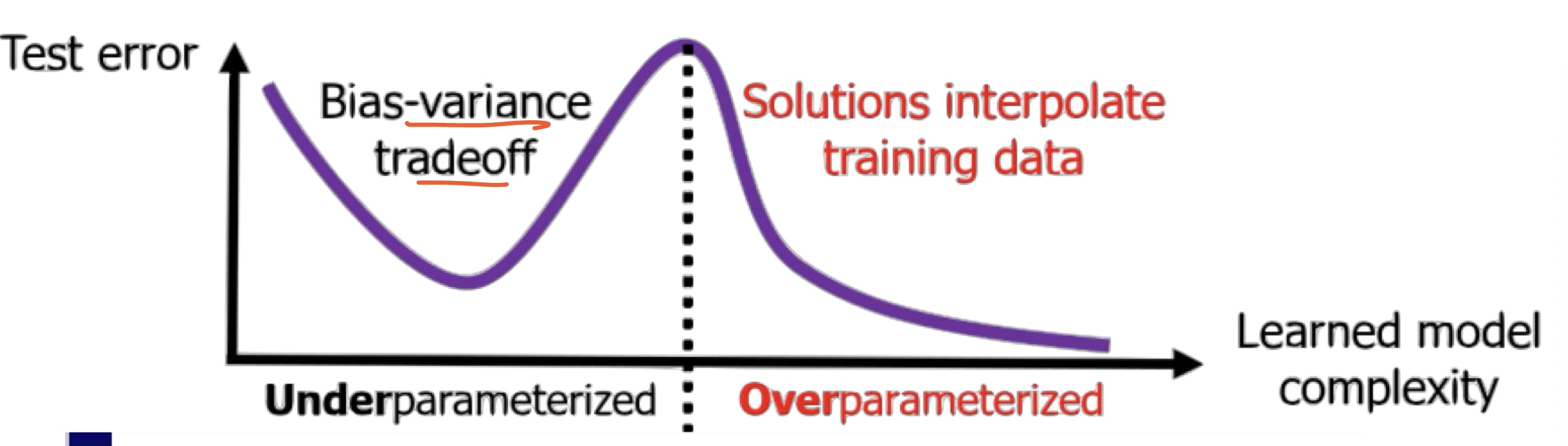
Classic U-curve (first descent).
As capacity increases from very small, Bias falls faster than Variance rises, so test error drops.

Interpolation peak.
Near the point where the model just fits training data exactly (interpolation), Variance spikes ⇒ test error peaks.

Second descent (overparameterized regime).
With even more capacity, test error falls again because learning dynamics and architecture steer solutions toward simpler interpolants:

Implicit regularization of SGD: among many perfect-fit solutions, training prefers low-norm/low-complexity ones.
Architectural inductive bias: convolutions/attention/residuals encode structures that generalize.
Scale with data: large datasets dampen variance and let capacity be used productively.

Which descent is “better”?

Linear regression (classic): often the first descent (pre-interpolation, $p<n$) achieves the lowest test error; the overparameterized second descent ($p\gg n$) may not beat it.
Deep learning (modern practice): typically the second descent (massively overparameterized) is better when there is enough data, SGD’s implicit bias, and good architectures/regularization. That’s why today larger models often generalize better.