Lecture 10
Regularization and Generalization
Today’s Topics:
- 0. From last lecture: Kaggle Cats & Dogs + DataLoader
- 1. Improving Generalization
- 2. Data Augmentation
- 3. Early Stopping
- 4. L1 and L2 Regularization
- 5. Dropout
0. From last lecture: Kaggle Cats & Dogs + DataLoader
Kaggle is a platform for hosting datasets and machine learning competitions. Organizations (companies, research groups, or nonprofits) upload datasets and define an evaluation metric. Participants train models and submit predictions; the best-performing models appear at the top of the leaderboard and may receive prizes.
Reference notebook (VGG16 on Cats vs. Dogs):
- https://github.com/rasbt/deeplearning-models/blob/master/pytorch_ipynb/cnn/cnn-vgg16-cats-dogs.ipynb
Why PyTorch Dataset and DataLoader are needed
Real-world datasets (especially images) are often too large to load into memory at once. PyTorch separates data handling into two components:
Dataset- Defines how to retrieve a single example.
- Maps an index
i→(x_i, y_i)(e.g., load image from disk, apply transforms, return label).
DataLoader- Wraps a Dataset and provides an iterator over mini-batches.
- Handles:
- batching (
batch_size) - shuffling (
shuffle=Truefor training) - parallel data loading (
num_workers) - efficient memory transfer (
pin_memory=Truewhen using GPUs)
- batching (
This design enables efficient, scalable training by streaming data batch-by-batch instead of loading the full dataset at once. Custom DataLoader example notebook:
- https://github.com/rasbt/stat453-deep-learning-ss20/blob/master/L08-mlp/code/custom-dataloader/custom-dataloader-example.ipynb
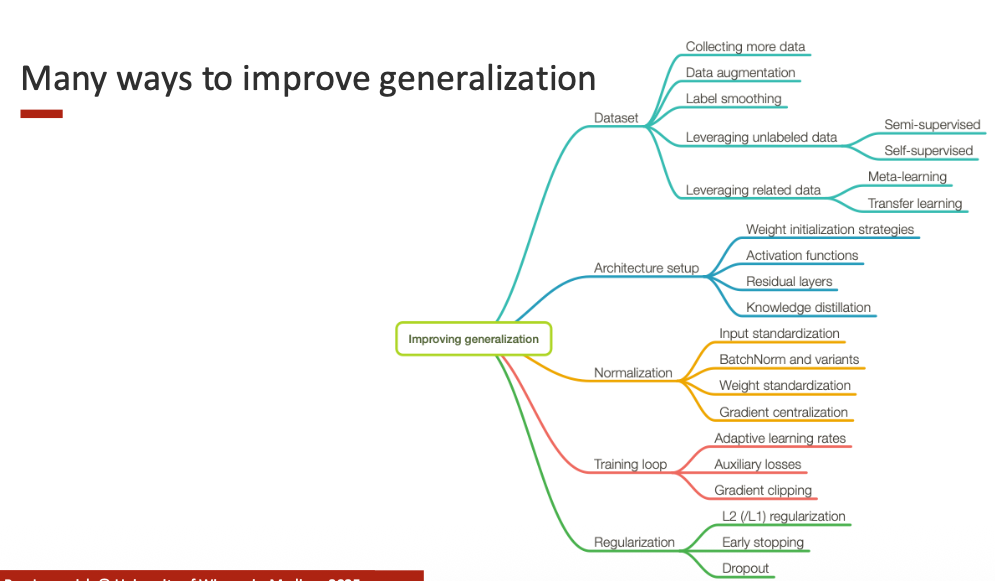
1. Improving Generalization
Generalization refers to how well a trained model performs on unseen data.
A model that generalizes well captures the true underlying patterns in the dataset instead of memorizing noise from the training set.
Achieving high training accuracy is not enough — the goal is to ensure that the model performs well on new data.
Overfitting occurs when a model is too closely tailored to the training set, leading to poor test performance.
Key strategies to improve generalization:
- Collect more diverse data
- Use data augmentation
- Reduce model capacity (simpler models)
- Apply regularization (L1, L2, dropout)
- Use early stopping
- Employ transfer/self-supervised learning
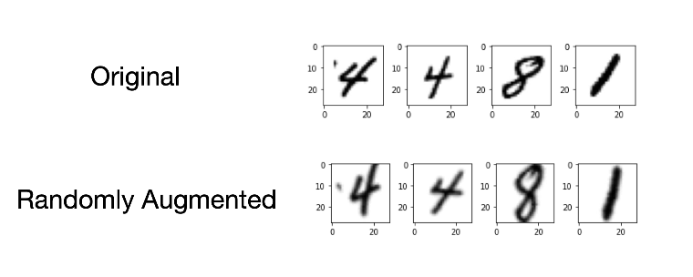
2. Data Augmentation
Data augmentation increases dataset size by generating label-preserving transformations — improving robustness and reducing overfitting.
Useful when labeled data is scarce or costly (e.g., medical imaging).
Common augmentations:
- Random crop / resize
- Flipping, rotation, translation, zoom
- Adding noise or color jitter
- Mixup, CutMix
These simulate real-world variations and encourage invariant feature learning.
3. Early Stopping
Reducing Model Capacity
Another way to improve generalization is to reduce the effective capacity of the model.
Common approaches include:
- Using smaller architectures (fewer layers or hidden units)
- Applying L1 or L2 regularization to penalize large weights
- Using dropout to randomly disable neurons during training
- Freezing most parameters in large pretrained models and fine-tuning only a small subset
In modern deep learning, it is common to start with a large pretrained model and control capacity through regularization and selective fine-tuning rather than training small models from scratch.
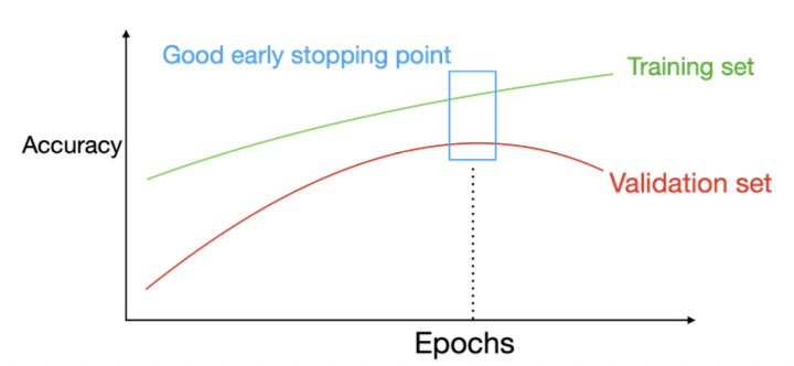
Early Stopping
Early stopping halts training when validation performance stops improving — preventing overfitting.
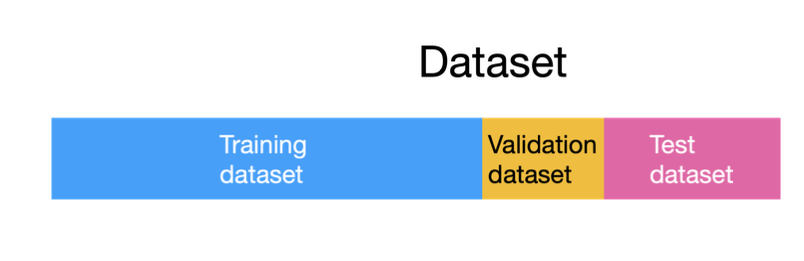
Procedure
- Split data into training/validation/test.
- Track validation performance.
- Stop training when validation loss stops decreasing.
4. L1 and L2 Regularization
Regularization penalizes large weights, encouraging simpler models and preventing overfitting.L1 regularization corresponds to LASSO, while L2 regularization corresponds to Ridge regression
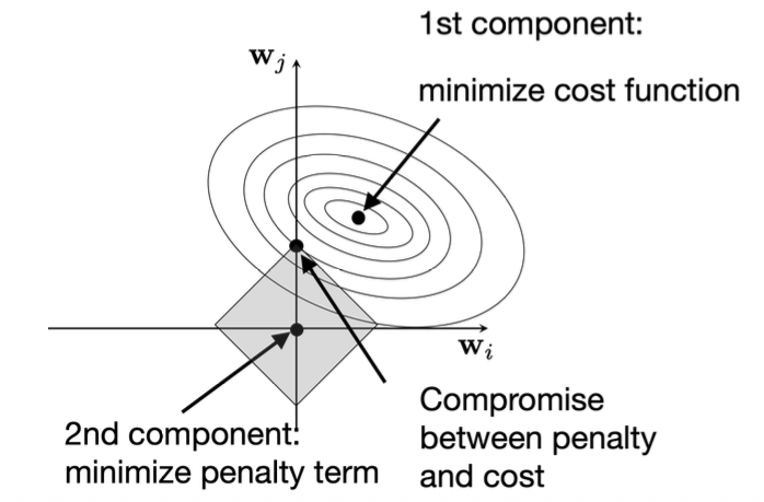
4.1 L1 Regularization (Lasso)
\(\mathcal{L}_{L1} = \frac{1}{n}\sum_{i=1}^{n} L(y^{[i]}, \hat{y}^{[i]}) + \frac{\lambda}{n}\sum_{j} |w_j|\)
-L1 Regularization (Lasso) adds the sum of the absolute values of all weights as a penalty term to the loss function, helping to control model complexity.
-It drives many weights to zero, producing a sparse solution and enabling automatic feature selection.
-Geometrically, the circular contours represent the cost function, while the diamond shape represents the L1 constraint boundary. The model seeks a balance between minimizing the loss and satisfying the constraint.
-Because the diamond has sharp corners that align with the coordinate axes, the optimal point often lies on an axis, causing some weights to become exactly zero.
-This regularization prevents overfitting and makes the resulting model simpler and more interpretable.
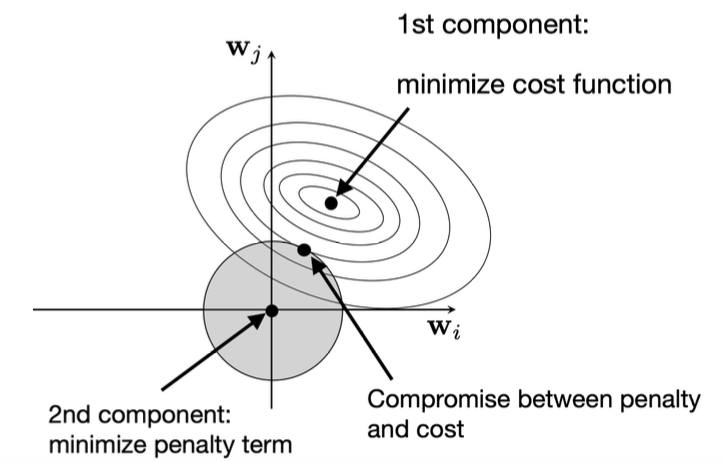
4.2 L2 Regularization (Ridge)
\[\mathcal{L}_{L2} = \frac{1}{n}\sum_{i=1}^{n} L(y^{[i]}, \hat{y}^{[i]}) + \frac{\lambda}{n}\sum_{j} w_j^2\]w_{i,j} := w_{i,j} - \eta!\left(\frac{\partial L}{\partial w_{i,j}} + \frac{2\lambda}{n}w_{i,j}\right) </d-math>
-L2 Regularization (Ridge) adds the sum of squared weights as a penalty term to the loss function, discouraging large coefficients.
-Unlike L1, it does not force weights to zero, but instead smooths them toward smaller values, distributing the influence more evenly among features.
-Geometrically, the circular contour lines represent the cost function, while the gray circle represents the L2 constraint.
-The optimal point lies where the cost contour just touches the constraint circle, balancing the trade-off between minimizing the cost and the penalty term.
-Because the circle has no sharp corners, all weights are shrunk but rarely become zero, which means L2 encourages weight smoothing rather than sparsity.
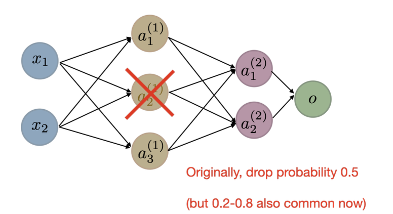
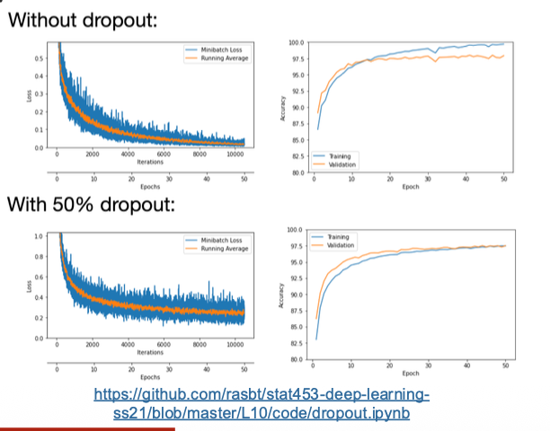
5. Dropout
Dropout randomly removes a fraction of neurons during training — forcing the network to learn redundant, distributed representations.
Why it works
- Prevents co-adaptation
- Acts like model ensemble
- Improves robustness
Summary
Regularization and generalization methods — like data augmentation, early stopping, L2, and dropout — are essential to ensure models learn meaningful patterns, not noise.
They enable robust generalization and stable performance on unseen data.