Lecture 11

Normalization / Initialization

Lecture Notes: Normalization and Initialization in Deep Learning

Based on lecture transcript and accompanying slides.
Topic: Normalization and Initialization (Gordon, Lecture 11).
Course context: Regularization, stability, and optimization in neural networks.

---

1. Research Projects and Reading Papers

1.1 Choosing a Project Direction

Before designing architectures (e.g., transformers), it is recommended to first decide on an application domain.

• Select an area of interest such as medical image analysis, speech recognition, or sequence modeling.
• Perform a literature review of approximately 10 recent papers within that field.
• Identify the model architectures and methods employed.
• Even without full comprehension, one can replicate or slightly modify those studies to form a meaningful project.

1.2 Critical and Optimistic Reading

Academic papers, even from leading institutions, invariably contain flaws. The productive mindset combines:

• Critical analysis: Identifying gaps, assumptions, or methodological weaknesses.
• Optimism and curiosity: Recognizing that “all papers are wrong, but some are useful.” This balance encourages innovation while maintaining intellectual humility.

---

2. Motivation for Normalization

2.1 Optimization Landscape Intuition

Training via gradient descent can be visualized as movement over a loss surface.

• Thus, if topological graph is warped, gradient descent will bounce around from tangent to tangent.
• Proper normalization produces a more isotropic (spherical) loss contour, ensuring direct descent toward the minimum.

2.2 Deep Learning Context

• Input features can be normalized directly.
• However, hidden layer activations evolve during training, altering their distribution dynamically.
• This motivates internal normalization techniques such as Batch Normalization.

---

3. Batch Normalization (BatchNorm)

3.1 Conceptual Overview

Proposed by Ioffe and Szegedy (2015), Batch Normalization addresses instability in training deep networks. It normalizes intermediate activations within each mini-batch to stabilize distributions. Backpropogating larger parameters in gradient descent creates large partial derivatives, and multiplying many of them form a larger & larger number; BatchNorm helps to deal with “exploding gradients”.

Essentially, these are additional layers on our models which improve stability and convergence rates.

Note: Assuming each minibatch is a node belonging to a given hidden layer, we are providing additional (normalization) information to each.

Given activations (z_i) for a layer across a mini-batch of size (n):

Normalizing Net Inputs:

\mu_B = \frac{1}{n}\sum_{i=1}^{n} z_i, \qquad \sigma_B^2 = \frac{1}{n}\sum_{i=1}^{n}(z_i - \mu_B)^2

• $\mu_B$ and $\sigma_B^2$ are not learnable

\hat{z}_i = \frac{z_i - \mu_B}{\sigma_B}

However, in practice the below equation is used for numerical stability:

\hat{z}_i = \frac{z_i - \mu_B}{\sqrt{\sigma_B^2 + \varepsilon}}

Affine transformation (learnable scaling and shifting):

y_i = \gamma \hat{z}_i + \beta

• $\gamma$ and $\beta$ are learnable parameters allowing the network to recover the optimal scale and bias.
  • $\gamma$ controls the spread
  • $\beta$ controls the mean
• An optimal activation distribution typically has zero mean and unit variance. Batch normalization standardizes activations to have zero mean and unit variance, improving training stability.
• This mechanism maintains flexibility while mitigating exploding or vanishing gradients.
• $\beta$ makes bias units redundant

Figure 1. batchnorm

---

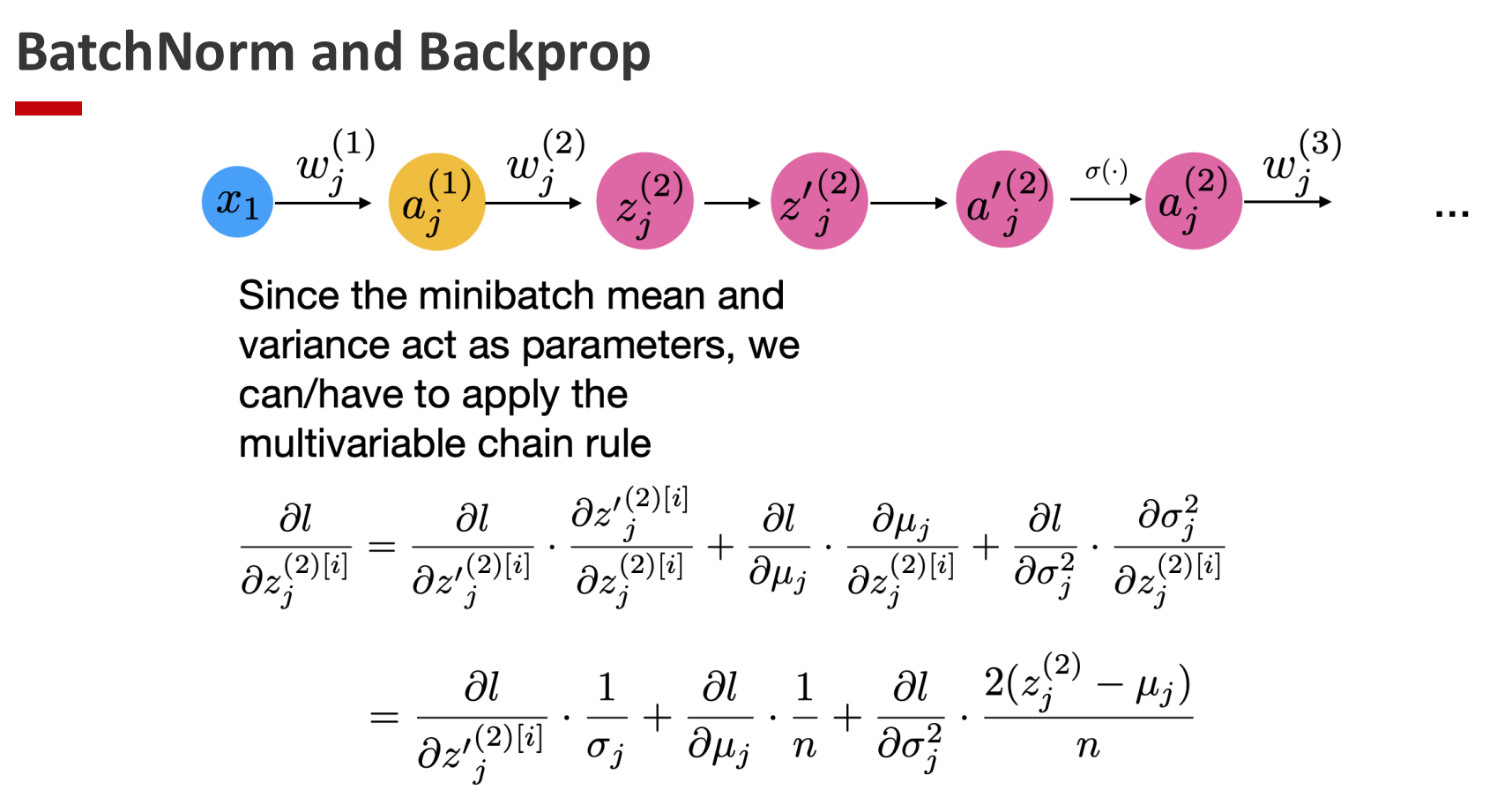
3.2 Learning BatchNorm Parameters

BatchNorm fits naturally into the computation graph:

1. Linear transformation: (z = Wx + b)
2. Normalization: (\hat{z})
3. Rescaling and shifting: (y = \gamma \hat{z} + \beta)
4. Nonlinear activation: (a = f(y))

Since all operations are differentiable, backpropagation proceeds seamlessly.

Figure 2. batchnorm nad backprop

---

---

3.3 Training vs. Inference

• Training phase: Uses mini-batch statistics ((\mu_B, \sigma_B^2)).
• Inference phase: Employs moving averages of (\mu) and (\sigma^2) accumulated during training. This ensures consistent behavior when batch sizes differ or when predictions are made one sample at a time.

---

3.4 BatchNorm in PyTorch

• Can add BatchNorm into model via simple torch.nn.BatchNorm1d/2d/3d(num_features)
• Based on summary statistics of the mini-batch, we can normalize before scaling
• Implement model.train() and model.test() before training and testing, respectively

---

3.5 Empirical Benefits

1. Accelerated convergence through more stable gradients.
   • The model has the same optimization without batch norm, but with a smoother learning rate, we can train more quickly
2. Mitigation of internal distribution shifts.
3. Enables higher learning rates and deeper networks.
4. Often improves generalization due to mild regularization effects.

---

3.6 Theoretical Explanations (Multiple Perspectives)

Year	Explanation	Source / Insight
2015	Internal Covariate Shift hypothesis	Original BN paper
2018–2019	Smoothing of optimization landscape	MIT study (Santurkar et al.)
2018	Implicit regularization effect	Empirical observations
2019	Stabilized gradient dynamics allowing larger learning rates	Theoretical reinterpretation

Despite differing theoretical justifications, all confirm that BN improves training stability and speed.

---

3.7 Practical Considerations

• Batch Size Sensitivity:
  • BatchNorm becomes more stable with larger mini-batches
  • To improve stability, we can introduce larger mini-batch sizes
• Order of operations: Commonly Linear/Conv → BatchNorm → ReLU; variations may be task-dependent.
• PyTorch Implementation: torch.nn.BatchNorm1d/2d/3d; ensure proper use of model.train() and model.eval().

• Alternative Normalization Methods:

  • Layer Normalization (LN): Across features of a single sample; suitable for sequence models and transformers.
    • Finds the mean and standard deviation based on feature vectors (while BN calculates mean/std based on mini-batch)
    • Applied to transformers

---

4. Initialization of Network Weights

4.1 Importance of Initialization

Improper initialization can result in:

• Symmetry among neurons (if all weights equal): we cannot initialize all weights to zero.
  • This is a problem because in fully connected layers nodes wouldn’t be differentiable
• Vanishing or exploding gradients, especially in deep networks. Therefore, initialization affects both convergence rate and final performance.

This results in the inability for hidden layers to be distingushed from one another, and prevents us from finding the optimal minima.

---

4.2 Xavier (Glorot) Initialization

Designed for activation functions centered near zero (e.g., tanh). Steps:

1. Initialize weights from Normal or Uniform distribution.
2. Scale weights proportional to the number of inputs to the layer.

W^{l} := W^{l} * \sqrt{\frac{1}{m^{l-1}}}

• m is the number of input units to the next layer

\begin{aligned} \mathrm{Var}\left(z_j^{(l)}\right) &= \mathrm{Var}\left(\sum_{k=1}^{m_{l-1}} W_{jk}^{(l)} a_k^{(l-1)}\right) \\ &= \sum_{k=1}^{m_{l-1}} \mathrm{Var}\left(W_{jk}^{(l)} a_k^{(l-1)}\right) = \sum_{k=1}^{m_{l-1}} \mathrm{Var}\left(W_{jk}^{(l)}\right) \mathrm{Var}\left(a_k^{(l-1)}\right) \\ &= \sum_{k=1}^{m_{l-1}} \mathrm{Var}\left(W^{(l)}\right) \mathrm{Var}\left(a^{(l-1)}\right) = m_{l-1} \, \mathrm{Var}\left(W^{(l)}\right) \mathrm{Var}\left(a^{(l-1)}\right) \end{aligned}

---

4.3 He (Kaiming) Initialization

Tailored for ReLU activations, which are non-symmetric around zero.

Same steps as in Xavier Initialization, but we add a factor of √2 when scaling weights:

W^{l} := W^{l} * \sqrt{\frac{2}{m^{l-1}}}

Reasoning:

W \sim \mathcal{N}\left(0, \frac{2}{n_{in}}\right)

This scaling compensates for the half-rectification effect of ReLU and maintains activation variance consistency.

• PyTorch default: Linear and convolutional layers use He initialization by default.

---

4.4 Architectural Dependence

The optimal initialization scheme may depend on:

• Network depth and width.
• Nonlinearity used.
• Presence of residual or skip connections. Deep architectures often rely on residual connections to alleviate gradient vanishing, beyond what normalization or initialization alone can achieve.

---

5. Gradient Stability and Residual Structures

To combat vanishing/exploding gradients:

• Introduce residual (skip) connections or scaled shortcuts that enable direct gradient flow.
• Such designs have become integral to modern architectures (e.g., ResNets, Transformers).

---

6. Implementation Summary

6.1 Normalization

Technique	Applied Axis	Common Use	Advantages	Limitations
BatchNorm	Across mini-batch	CNNs	Fast convergence	Requires large batch
LayerNorm	Across features	Transformers	Batch-independent	Slightly slower
InstanceNorm	Across spatial dims	Style transfer	Instance-specific	Limited effect on stability
GroupNorm	Across channel groups	Small-batch CNNs	Stable	Needs tuning of group size

---

6.2 Initialization Quick Reference

Scheme	Suitable Activation	Formula	Key Idea
Xavier (Glorot)	tanh / sigmoid	Var(W)=1/(n_{in}+n_{out})	Equalize activation variance
He (Kaiming)	ReLU / LeakyReLU	Var(W)=2/n_{in}	Compensate for ReLU truncation

---

7. Key Takeaways

1. Normalization stabilizes internal representations, accelerates convergence, and improves training reliability.
2. BatchNorm remains the most effective and widely used technique despite incomplete theoretical justification.
3. Initialization directly influences optimization trajectory; Xavier and He methods are standard baselines.
4. Residual connections further enhance gradient flow, crucial for very deep models.
5. Understanding and controlling the interplay between normalization, initialization, and architecture is central to modern deep learning engineering.

---