Lecture 12

Improving Optimization

Today’s Topics:

[1. Midterm]

[2. Learning Rate Decay:]

[3. Learning Rate Schedulers in PyTorch:]

[4. Training with “Momentum”:]

[5. ADAM: Adaptive Learning Rates]

[6. Optimization Algorithms in PyTorch]

---

1. Midterm

• In-class on Wednesday, 10/22
• Open-note, no electronics/AI
• Review Session on 10/20; study guide released 10/13
• Types of Questions:
  • True/False
  • Multiple Choice
  • Derivation
  • Matching algorithms to property
  • Interpreting Python code blocks

Content:

• Lecture materials
• Readings are designed to support learning, but will not be tested directly on midterm

---

2. Learning Rate Decay:

• Minibatch Training Recap:

  • Minibatch learning is a form of stochastic gradient descent

  • Each minibatch is a sample drawn from the training set and the training set is in turn a sample drawn from the population. Model output, loss, and gradient is calculated for each minibatch.

  • Minibatch helps minimize computational cost with fullbatch gradient descent, but creates a noiser gradient due to increased oscillation.
    • Smaller batches creates noisier gradient.
  • Noiser gradients are helpful in non-convex landscapes to escape local minima
• Noise is a double-edged sword:
  • Good: helps escape local minima.
  • Bad: causes oscillation.
• Minibatch Training: Practical Tip
  • Typical minibatch sizes: 32, 64, 128, 256, 512, 1024 to correspond with memory bytes
    • Pick the largest minibatch that is allowed by GPU memory

  • Nice to match the batch size to the number of class sizes in the dataset because want to have the minibatches perserve the distribution of labels from the population in the minibatch sample.

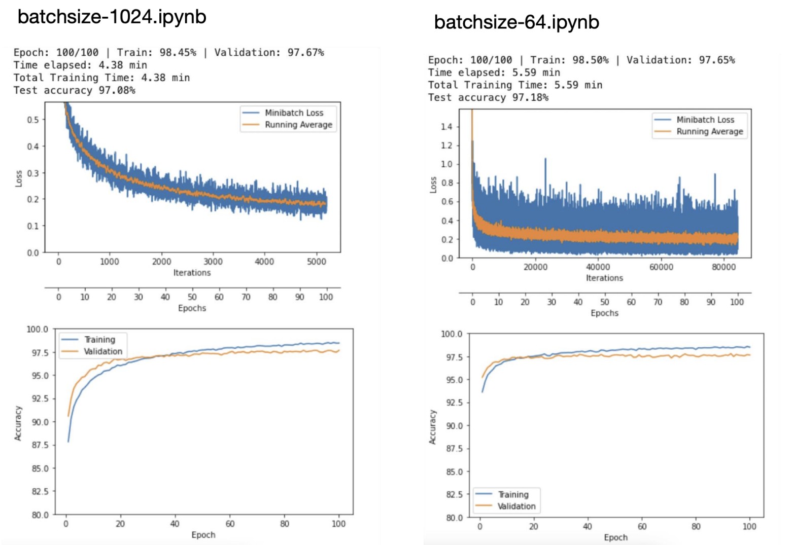
  • Smaller batches → noisier gradients → more loss oscillation but similar final accuracy.

  • In Figure 1 below, more loss oscillation with the smaller batches sizes, but the accuracy is similar.

Figure 1. Visualization shown during Lecture 12.

• Learning Rate Decay:

  • Minibatches are samples of the training set, so loss and gradients from the minibatches are approximations. This creates oscillations.

  • To decrease oscillations, we can decay the learning rate to prevent missing the true minimum.

  • On a practical note, train model without learning rate decay and then fit the decay to what is observed. This avoids decaying too fast and missing the minimum. This can also be done through validation set testing.

    • Follows the idea of deep learning to overfit model and then fix the model. This proves the features can model the data.
• Equations of Learning Rate Decay:
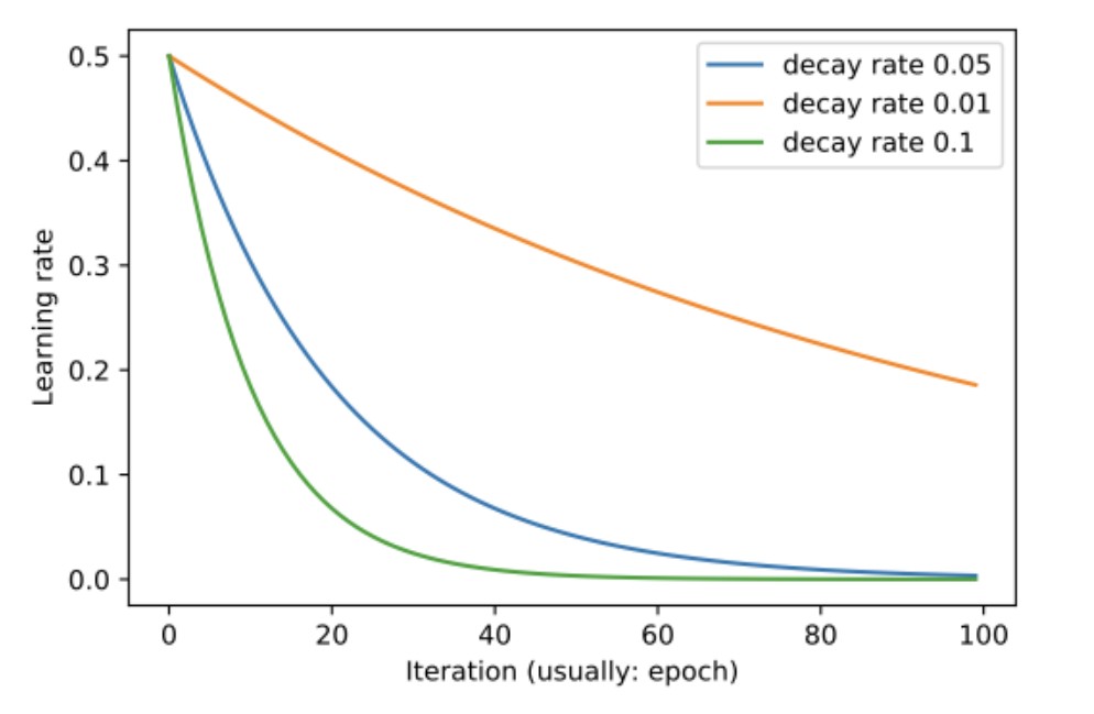
  • Exponential Decay:
    • $\eta_t=\eta_0 e^{-k\cdot t}$

      • $\eta$ is the learning rate

      • $k$ is the hyperparameter of the decay

      • $t$ is the epochs

      • Figure 2 shows that by 100 epochs the learning is drastically different between orange and green/blue:

Figure 1. Visualization shown during Lecture 12.

• Learning Rate and Batch Size:
  • Can get identical accuracy by increasing batch size rather than decreasing learning rate. However, this goes against the initial problem that learning rate decay solves: GPU and memory costs.

Common Forms of Learning Rate Decay

Type	Formula	Notes
Exponential Decay	$\eta_t = \eta_0 e^{-k t}$	Smooth continuous decay; $k$ is rate hyperparameter
Step (Halving)	$\eta_t = \eta_{t-1}/2$ every $T_0$ epochs	Simple, common in classification
Inverse Decay	$\eta_t = \frac{\eta_0}{1 + k t}$	Slower decay, often more stable

⚖️ Key idea: Decay reduces update magnitude so the model “settles” near the minimum instead of bouncing around.

---

---

3. Learning Rate Schedulers in PyTorch:

• [Option 1:]{.underline} Call your own junction at the end of each epoch:

• [Option 2:]{.underline} Use one of the built-in tools in PyTorch.
  1. The “torch.optim.lr.scheduler.LambdaLR” is the most common, generic version
• Saving Models in PyTorch:

  • The model, optimizer, and the tearning rate scheduler all have save functionalities in PyTorch. This is essential for reuse and reproducability.

  • torch.save(model.state_dict(), “…”)

  • torch.save(optimizer.state_dict(), “…”)

  • torch.save(scheduler.state_dict(), “…”)

---

4. Training with “Momentum”:

• The main idea of momentum is to dampen oscillations by using “velocity” which is the speed of the “movement” from previous updates. This helps skip over local minima by increasing efficiency.

• Key take-away: not only move in the direction of the gradient, but also move in the “weighted averaged” direction of the last few updates.

  Gradient $\Delta w_{i,j}(t)$ is the “velocity” $V$:

  $\Delta w_{i,j}(t) := \alpha \cdot \Delta w_{i,j}(t-1) + \eta \cdot \frac{\partial l}{\partial w_{i,j}}(t)$

  • $\alpha$ is the momentum parameter, usually a value between 0.9 and 0.99. This is like a “friction” or dampening parameter.

  • $\Delta w_{i,j}(t-1)$ update at the previous step

  • $\eta \cdot \frac{\partial l}{\partial w_{i,j}}(t)$ familiar, regular gradient update

    • We “average” this by adding it to the previous update.
• In PyTorch:
  • “torch.optim.SGD(params, lr=<required parameter>, momentum=0, dampening=0, weight_decay=0), nesterov=False.
    • dampening $1-\eta$, how much do you dampen your current minibatch update.
• Nesterov: A Better Momentum
  • Given that we know the direction the momentum term will push us (because it was calculated by the previous term), we can skip ahead by applying the previous term’s momentum and then calculating loss with the momentum:

    • Before: $\Delta w(t) := \alpha \cdot \Delta w_{t-1} + \eta \cdot \Delta _w L (w_t)$

      $w_{t+1}:=w_t-\Delta w_t$

    • Nesterov: $\Delta w(t) := \alpha \cdot \Delta w_{t-1} + \eta \cdot \Delta w L (w_t - \alpha \cdot \Delta w{t-1})$

      $w_{t+1}:=w_t-\Delta w_t$

      • applying momentum term first because it was already calculated in the previous iteration.

Figure 1. Visualization shown during Lecture 12.

---

5. ADAM: Adaptive Learning Rates

• So far: decrease learning if the gradient changes its direction and increase learning if the gradient stays consistent

  • Step 1: Define a local gain $(g)$ for each weight (initialized with $g=1$):

    $\Delta w_{i,j}:=\eta\cdot g_{i,j}\cdot\frac{\partial L}{\partial w_{i,j}}$

  • Step 2:

    • If gradient is consistent: $g_{i,j}(t) := (t-1)+ \beta$

    • Else: $g_{i,j}(t) := (t-1) \cdot (1-\beta)$

      • We multiply so that $g$ does not go negative, but decreases
• RMSProp is an algorithm created by Geoff Hinton that is similar to AdaDelta.

  • RMS is “Root Mean Squared” and divides the learning rate by an exponentially decreasing moving average of the squared gradients.

  • It takes into account that gradients can vary widely in magnitude and damps oscillations like momentum

• ADAM:
  • Most widely used optimization algorithm in DL and combines momentum and RMSProp.

    • [Momentum-like Term:]{.underline}$\Delta w_{i,j}(t) := \alpha \cdot \Delta w_{i,j}(t-1) + \eta \cdot \frac{\partial l}{\partial w_{i,j}}(t)$

      This is written as:$m_t := \alpha \cdot m_{t-1}+(1-\alpha) \cdot \frac{\partial l}{\partial w_{i,j}}(t)$

    • [RMSProp Term:]{.underline}

      $r:= \beta \cdot MeanSquare(w_{i,j},t-1)+(1-\beta)(\frac{\partial L}{\partial w_{i,j}(t)})^2$

      • $r$ is the size of the gradients (large $r$ is steep)

    • [ADAM Update:]{.underline}

      $w_{i,j} := w_i,j - \eta \frac{m_t}{\sqrt{r} + \epsilon}$

---

6. Optimization Algorithms in PyTorch

• One of the simplest optimizers is SGD. For example: torch.optim.SGD(model.parameters(), lr=0.01, momentum=0.9) The momentum term helps smooth the updates so the training process doesn’t shake too much when the gradient changes quickly.

• Another optimizer we use a lot is Adam: torch.optim.Adam(model.parameters(), lr=0.0001) Adam basically combines ideas from Momentum and RMSProp, which is why it usually works well without too much tuning.
  • A more complete version looks like: torch.optim.Adam(params, lr=0.001, betas=(0.9, 0.999), eps=1e-08) The two values in betas control how fast the moving averages of the gradients (and squared gradients) decay over time.
    • Inside the RMSProp-style update in Adam:
      0.9 corresponds to α,
      0.999 corresponds to β.
  • If you are using an optimizer that keeps internal state (like momentum or Adam), remember to save and load the optimizer state when you resume training. Otherwise, the optimizer will forget where it left off.
• Interesting hypothesis about ADAM, everything in machine learning has been engineered around ADAM because of how convenient it is as an optimizer. It may not give the best performance, but defaults give the a reliable, solid performance.

---