Lecture 13
Convolutional Neural Networks
Today’s Topics:
- 1. What CNNs Can Do
- 2. Image Classification
- 3. CNN Basics
- 4. Cross-Correlation vs Convolution
- 5. CNNs & Backpropagation
- 6. CNNs in PyTorch
1. What CNNs Can Do
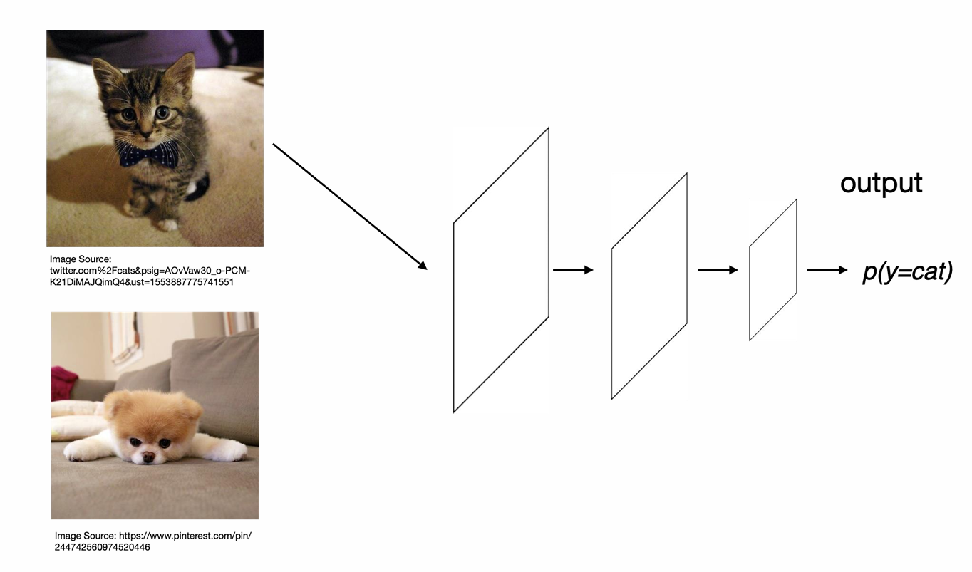
Image Classification
Definition: Assigning a single label to an entire image from a set of predefined categories.
Key Characteristics:
- Input: Entire image
- Output: Single class label with confidence score
- Question Answered: “What is the main object in this image?”
Examples:
- Classifying an image as “cat” vs “dog”
- Identifying handwritten digits (0-9)
- Medical image diagnosis (normal vs abnormal)
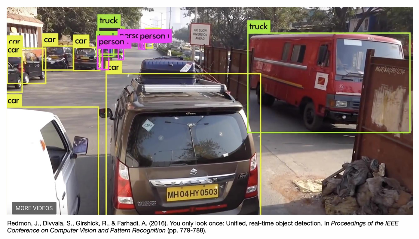
Object Detection
Definition: Identifying and localizing multiple objects within an image, including their positions and classifications.
Key Characteristics:
- Input: Entire image
- Output: Multiple bounding boxes + class labels
- Question Answered: “What objects are where in this image?”
Examples:
- Detecting cars, trucks, pedestrians in autonomous driving
- Finding faces and facial features in photos
- Inventory counting in retail
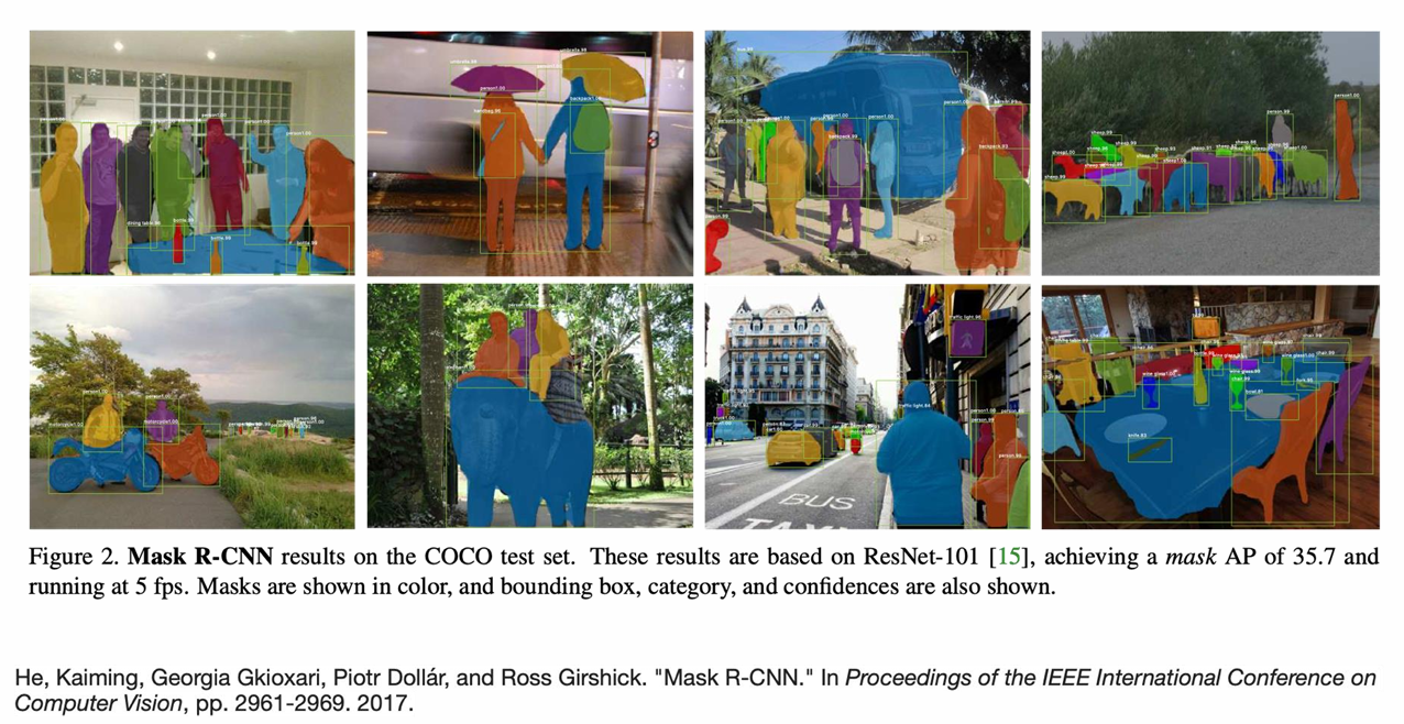
Object Segmentation
Definition: Pixel-level classification where each pixel in the image is assigned to a specific object category.
Key Characteristics:
- Input: Entire image
- Output: Pixel-wise mask with class labels
- Question Answered: “Which pixels belong to which objects?”
Types of Segmentation:
- Semantic Segmentation:
- Labels each pixel with a class
- Doesn’t distinguish between object instances
- Example: All “car” pixels get same label
- Instance Segmentation:
- Identifies and separates individual object instances
- Example: Differentiates between car1, car2, car3
Examples:
- Medical imaging (tumor boundary detection)
- Autonomous driving (road, pedestrian, vehicle segmentation)
- Photo editing tools (background removal)
2. Image Classification
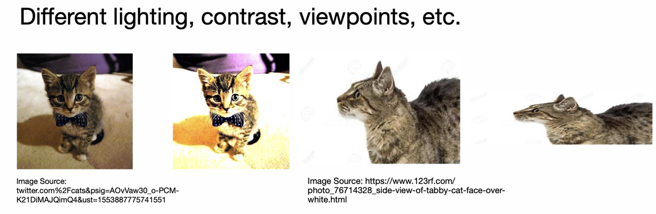
Why Images Are Hard for Neural Networks
1. Visual Variations
- Lighting changes: Same object under different illumination
- Contrast differences: Varying color and brightness levels
- Viewpoint variations: Objects seen from different angles
- Background clutter: Objects in complex environments
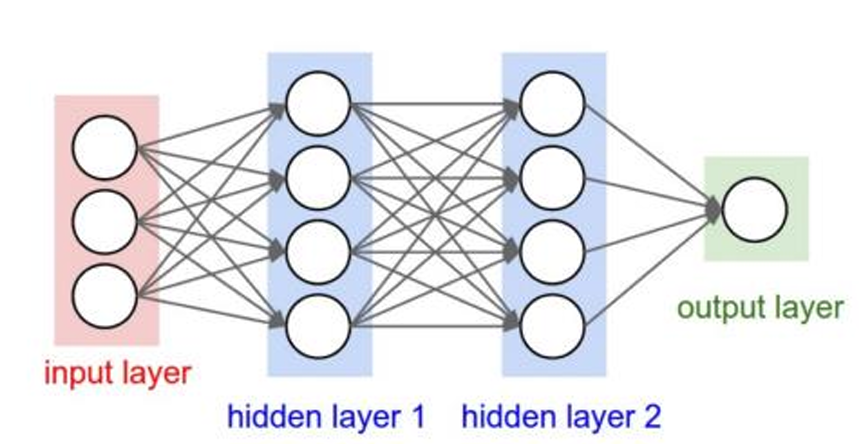
2. The Limitations of Fully-Connected Networks
- For a 3×200×200 RGB image: 120,000 input pixels. Each neuron in first hidden layer needs 120,000 weights
- Multiple hidden layers → parameter explosion
- In principle, a fully connected network has the capacity to approximate the mapping from raw pixels to labels, but in practice this quickly becomes impractical: the number of parameters grows linearly with the number of input pixels in every hidden unit and layer. By contrast, a CNN uses small filters (e.g., 3×3, 5×5) whose number of weights is independent of the input image size. The same filter is reused across all spatial positions, which dramatically reduces the parameter count and makes learning on high-dimensional image data feasible.
3. CNN Basics
Convolutional Neural Networks (LeCun 1989)
Core Idea: Parameter Sharing
- Instead of learning weights specific to absolute positions, learn weights defined for relative positions.
- Learn “filters” that are reused across the entire image.
- This allows the network to generalize across spatial translation of the input (e.g., recognize an object whether it’s in the top-left or bottom-right).
Key Mechanism:
- Replace traditional matrix multiplication with a convolution operation.
- This concept can be extended beyond images to graph-structured data.
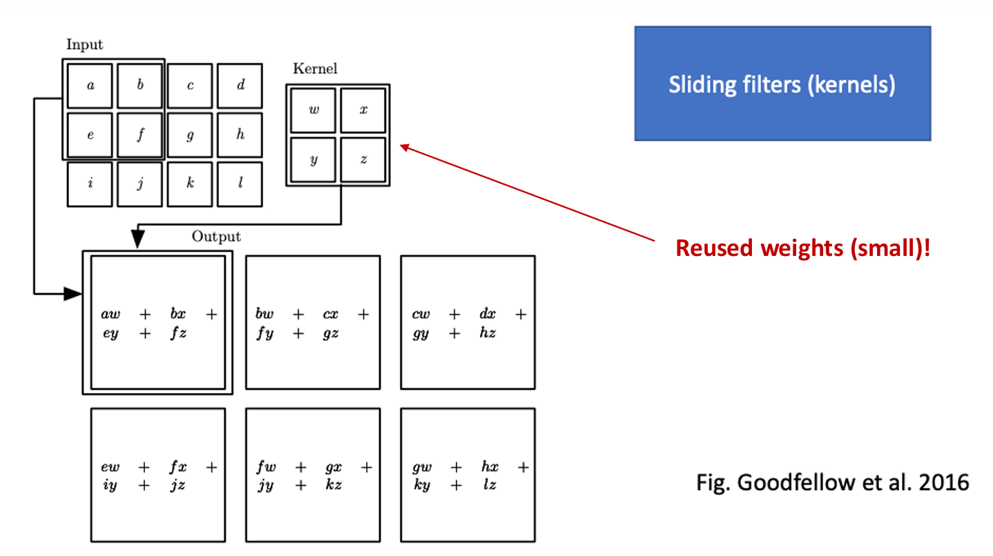
Weight Sharing in Kernels
How it works: A kernel (a small matrix of weights, e.g., $w, x, y, z$) acts as a sliding filter.
- Parameter Re-use: These weights are reused at every position as the filter slides over the input.
- Output Generation: The output (part of a “feature map”) is calculated by applying the kernel’s weights to the corresponding input values at each position (e.g., $aw + bx + ey + fz$).
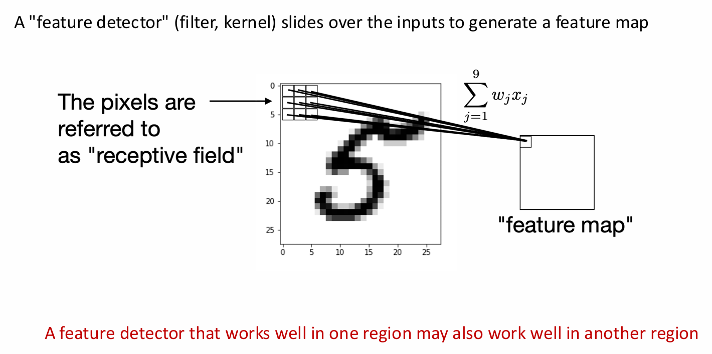
Alternative Visualization of Kernels
Concept: A “feature detector” (the filter or kernel) slides over the input image (like the “5”) to generate a “feature map”.
- Receptive Field: The specific patch of pixels the kernel is looking at at any given moment is called the “receptive field”.
- Calculation: Each value in the “feature map” is computed as a weighted sum (dot product) of the kernel’s weights ($w_i$) and the pixel values ($x_i$) within its receptive field: $\sum w_i x_i$.
- Guiding Principle: A feature detector that works well in one region (e.g., detects a curve) may also work well in another region.
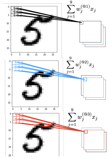
Kernels for each channel
Multiple feature detectors (kernels) can be applied in parallel to the same input image.
Each kernel learns different weights, producing different feature maps that highlight distinct aspects of the image.
- Each channel of the input (e.g., R/G/B for color images) has its own set of kernel weights.
- The outputs across channels are summed to produce the final feature map.
- This allows the network to combine local information across multiple input channels.
- Key idea: sparse connectivity and weight sharing are still preserved, even with multiple kernels.
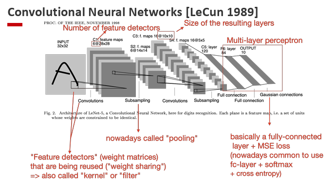
Convolutional Neural Networks [LeCun 1989]
LeCun and colleagues pioneered the use of Convolutional Neural Networks (CNNs) for digit recognition.
Their architecture, known as LeNet-5, combined convolutional feature extraction with traditional fully connected classifiers.
Key insights:
- Automatic feature extraction: Convolution + subsampling layers automatically learn and compress spatial features from raw pixel input.
- Regular classifier at the end: Fully connected layers + output layer act like a standard neural net classifier.
- Weight sharing: Filters (kernels) are reused across the input, drastically reducing the number of parameters.
- Pooling (subsampling): Early versions used average pooling to downsample feature maps and add robustness to shifts.
- Hierarchical learning: Local patterns → combined into higher-level features → final object recognition.
Network structure (LeNet-5 example):
- Input: 32×32 image.
- C1: Convolutional layer → 6 feature maps of size 28×28.
- S2: Subsampling (pooling) layer → 6 maps of size 14×14.
- C3: Convolutional layer → 16 maps of size 10×10.
- S4: Subsampling layer → 16 maps of size 5×5.
- C5: Convolutional layer → 120 feature maps of size 1×1.
- F6: Fully connected layer → 84 units.
- Output: 10-way classifier with Gaussian (later replaced by softmax).
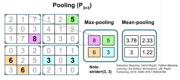
“Pooling”: lossy compression
Pooling layers reduce the dimensionality of feature maps while retaining the most important information.
This introduces translation invariance, helps control overfitting, and lowers computational cost.
Types of pooling:
- Max pooling: selects the maximum value from each region.
- Mean (average) pooling: computes the average value from each region.
Key points:
- Pooling operates over small, non-overlapping windows (e.g., 3×3).
- The stride determines how the window moves across the input (e.g., stride = (3,3)).
- Some information is discarded in the process, which is why pooling is considered lossy compression.
Main ideas of CNNs
Convolutional Neural Networks are built around three core principles:
- Sparse connectivity:
- Each element in the feature map is connected only to a small patch of the input (the receptive field).
- This is very different from fully connected networks, where each output is connected to all inputs.
- Key point: don’t connect everything to everything — only local regions are connected.
- Parameter sharing:
- The same weights (a kernel/filter) are reused for different patches of the input.
- This reduces the number of parameters and enforces translation invariance (the same feature can be detected anywhere in the input).
- Many layers:
- Stacking multiple convolution and pooling layers reduces the spatial size of the representation.
- Local features are gradually combined into global patterns.
- Finally, a multilayer perceptron (MLP) is placed on top to map the compact feature representation into predictions (e.g., class labels).
4. CC vs Convolution
Convolution: Adding two random variables
Convolution also appears in probability theory, when adding two independent random variables.
- Suppose $X \sim P_X, \; Y \sim P_Y$ are independent.
- What is $P(X+Y=z)$?
Continuous case:
\[P(X+Y=z) = \int P_X(x) P_Y(z-x) \, dx\]This integral is called the convolution of $P_X$ and $P_Y$:
\[(P_X * P_Y)(z) = \int P_X(x) P_Y(z-x)\, dx\]For discrete random variables, convolution is defined using a summation:
\[(P_X * P_Y)(z) = \sum_x P_X(x) P_Y(z-x)\]More generally:
- Discrete: $P_{X+Y}(z) = \sum_x P_{X,Y}(x, z-x)$
- Continuous: $f_{X+Y}(z) = \int f_{X,Y}(x, z-x)\, dx$
In CNNs, convolution is not about probability, but the same mathematical operation is reused.
- A kernel (filter) slides across the activation window.
- At each location, the kernel performs a weighted sum (dot product) of the overlapping region.
Formally:
\[Z[i,j] = \sum_{u=-k}^k \sum_{v=-k}^k K[u,v] \, A[i-u, j-v]\]Which is written compactly as:
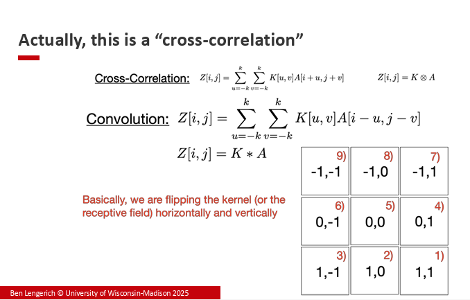
\[Z[i,j] = K * A\]Cross-Correlation vs. Convolution
In practice, most deep learning libraries (e.g., PyTorch, TensorFlow) actually implement cross-correlation rather than strict convolution.
-
Cross-correlation:
\[Z[i,j] = \sum_{u=-k}^k \sum_{v=-k}^k K[u,v] \, A[i+u, j+v]\] -
Convolution: \(Z[i,j] = \sum_{u=-k}^k \sum_{v=-k}^k K[u,v] \, A[i-u, j-v]\)
Key difference:
- Convolution flips the kernel horizontally and vertically before sliding.
- Cross-correlation uses the kernel as-is.
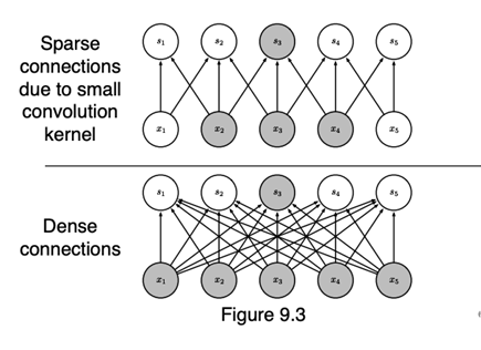
Sparse Connectivity in CNNs
Unlike fully-connected layers, CNNs use local connectivity:
- Each neuron in the feature map connects only to a small patch of the input (defined by the kernel size).
- This drastically reduces the number of parameters compared to dense connections.
- Sparse connections also enforce the idea that local patterns (e.g., edges, corners) are important for building up more complex representations.
Receptive Fields
Although each neuron starts with a local receptive field, stacking multiple convolution layers expands the effective receptive field:
- Lower layers capture small/local features (edges, corners).
- Higher layers combine these into larger/more abstract features (shapes, objects).
- This hierarchical growth enables CNNs to represent both local and global patterns.
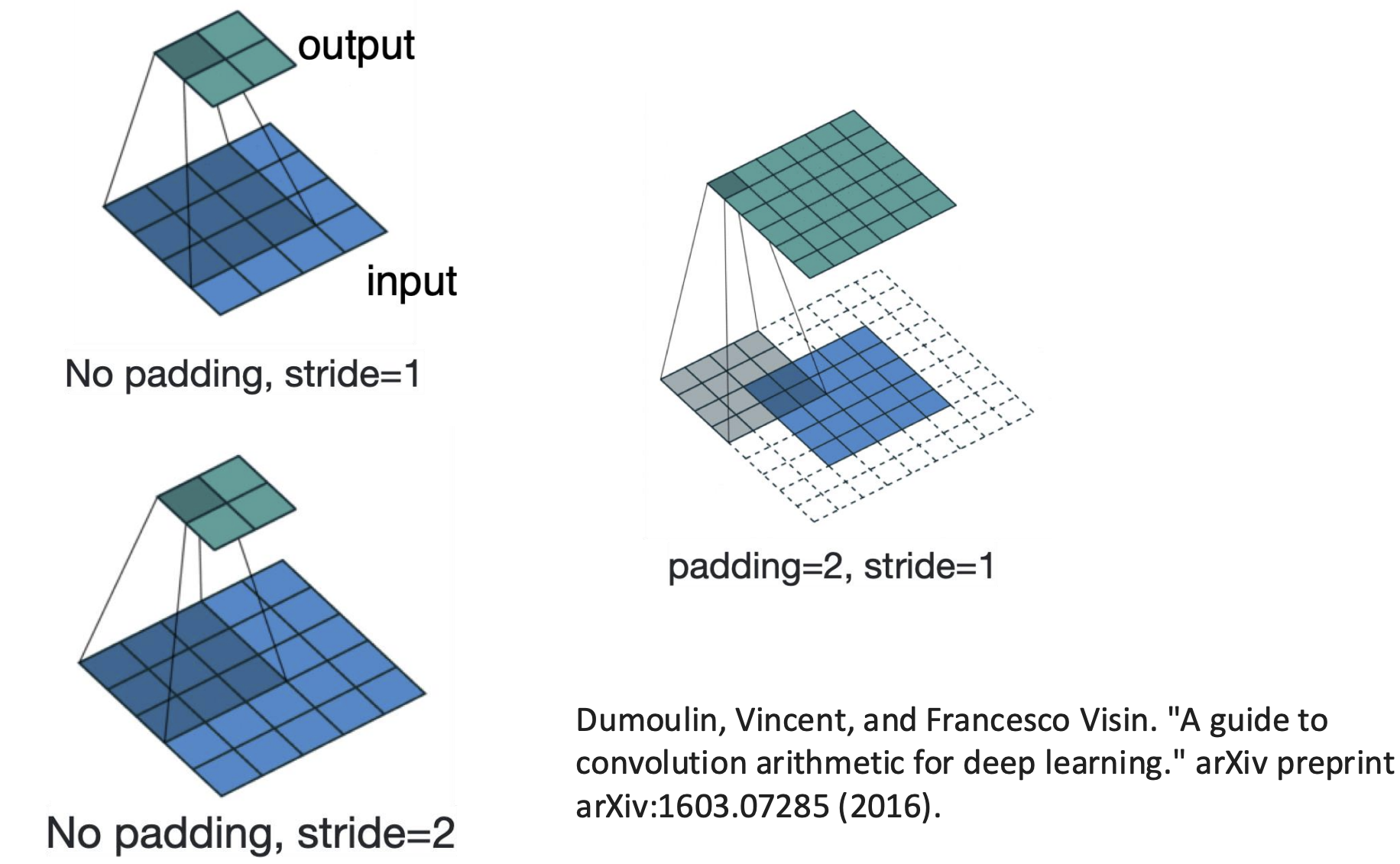
Impact of convolutions on size
The side length O of the feature map is below:
\[O = \frac{W-K+2P}{S}+1\]Where:
- W: input width
- K: kernel width
- P: padding
- S: stride
Below is a graph showing padding and stride:
Kernel dimensions and trainable parameters
-
For example, a convolutional layer has 3 input channels, 8 kernels, a kernel size of 5 × 5, and a stride of (1,1). Each kernel has dimensions 5 × 5, so the total number of trainable parameters is 5 × 5 × 3 × 8.
-
For a 28 × 28 input image, using a convolutional layer with a 5 × 5 kernel and stride of 1, the output size will be 24 × 24.
CNNs and Translation/Rotation/Scale Invariance
- CNNs are not inherently invariant to translation, rotation, or scale. Consequently, applying data augmentation by shifting, rotating, or scaling images can make CNN more robust during CNN training.
- In practice, CNNs provide only local / weak translation invariance: weight sharing and pooling make the network less sensitive to small shifts within a receptive field, but the activations still depend on where a pattern appears in the image overall. This is why CNNs can still be sensitive to small perturbations and even adversarial examples, despite using convolution and pooling.
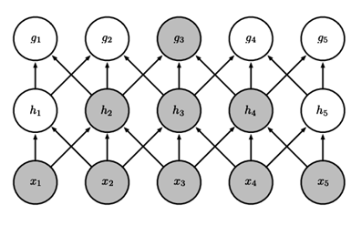
5. CNN Backprop
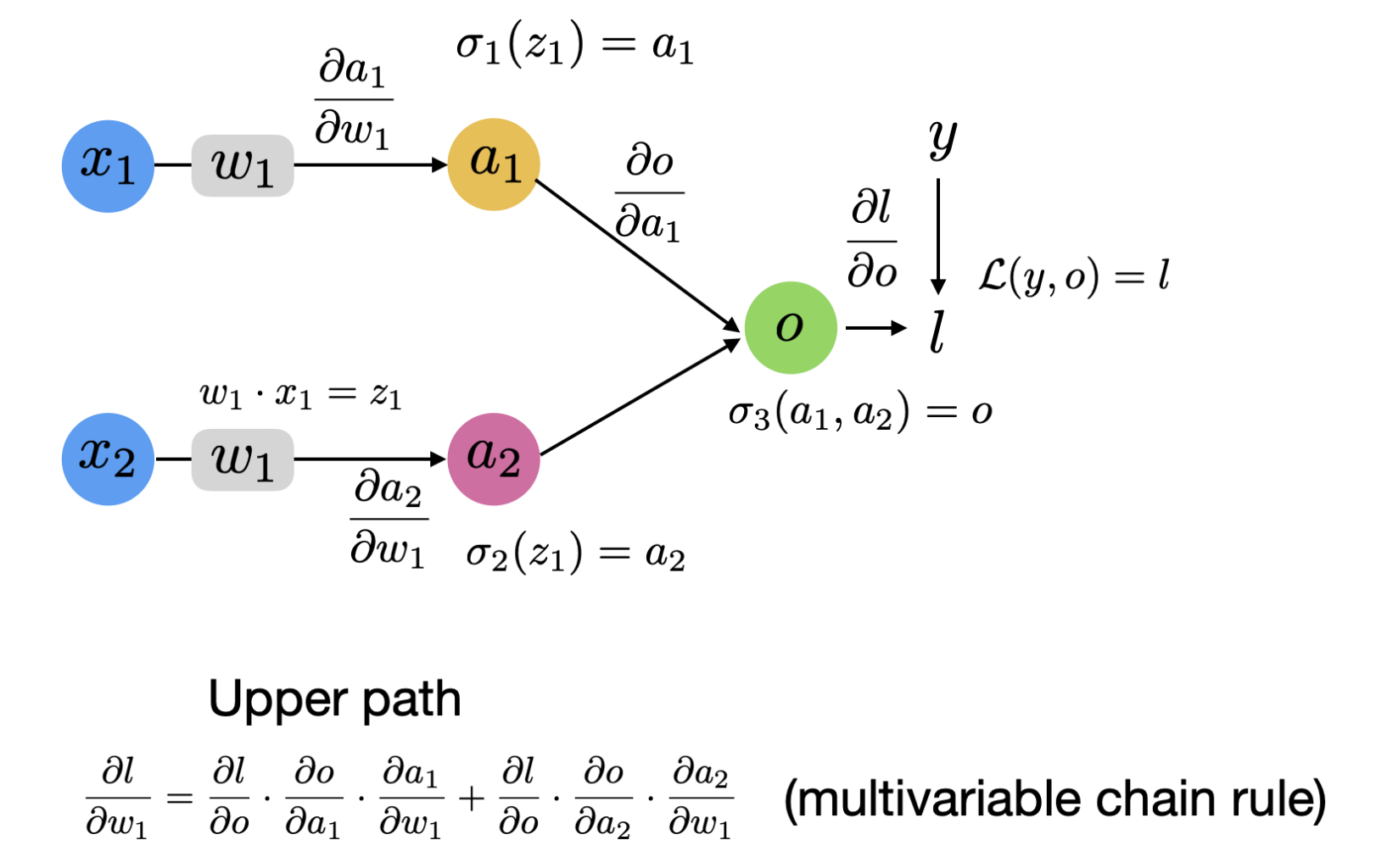
- In the computation graph, x: input. w: kernel weights. a: activation output. o: fully connected layer output. l: loss function.
- By $y = X * W + b$ we can derive that $\frac{\partial{L}}{\partial{W}} = X * \frac{\partial{L}}{\partial{y}}$
- the operator * means the sum of multiplication of two matrice’s corresponding entry.
mean of gradient
- For each kernel, there are multiple receptive fields in the input. For instance, a 3 × 3 kernel applied to a 5 × 5 input produces 4 receptive fields. During backpropagation, we compute the gradient for each receptive field and then take the average to update the kernel weights. \(w = w - \eta*\frac{\frac{l}{w}_1+\frac{l}{w}_2+\frac{l}{w}_3+\frac{l}{w}_4}{4}\)
- the same kernel weight is reused at many spatial locations, so its gradient is the sum of the contributions from all those locations. Backprop does not “break” for CNNs — we simply accumulate all the partial derivatives for the shared weight and then apply one update.
6. CNN PyTorch
-
in_channels: 1 for grayscale images, 3 for RGB images.
-
nn.Sequential: a container that holds all layers of the model; can often be used instead of explicitly defining a forward() function.
-
nn.Conv2d: a two-dimensional convolutional layer.
-
nn.MaxPool2d: a two-dimensional max pooling layer.