Lecture 14
Midterm Review
Table of Contents
- What is Machine Learning?
- The Building Blocks of Deep Learning
- Rosenblatt’s Perceptron
- Logistic Regression
- Multilayer Perceptron
- Backpropagation: An Algorithm to Train Models with Hidden Variables
- PyTorch: Automated Differentiation
- Improvements to Optimization
- Regularization
- Normalization
1. What is Machine Learning?
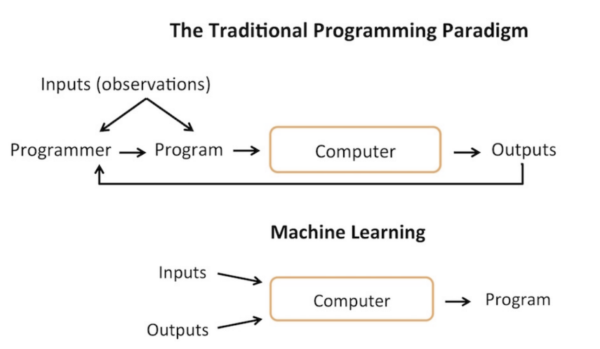
Machine learning is using statistically based methods to improve a model through its inputs and outputs.
Definition and Types
Formally, a computer program is said to learn from experience $E$ with respect to some task $T$ and performance measure $P$ if its performance at $T$ as measured by $P$ improves with $E$.
Supervised Learning
- Task $T$: Learn a function $h : X \to Y$
- Experience $E$: Labeled samples ${(x^{(i)}, y^{(i)})}_{i=1}^n$
- Performance $P$: A measure of how good $h$ is
Unsupervised Learning
- Task $T$: Discover structure in data
- Experience $E$: Unlabeled samples ${x^{(i)}}_{i=1}^n$
- Performance $P$: Measure of fit or utility
Reinforcement Learning
- Task $T$: Learn a policy $\pi : S \to A$
- Experience $E$: Interaction with environment
- Performance $P$: Expected reward
The Connection Between Fields
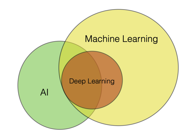
The relationship between artificial intelligence, machine learning, and deep learning can be understood hierarchically. AI represents a system that accomplishes a task through a machine learning or deep learning model. Machine Learning uses statistically based methods to improve a system’s performance through the inputs and outputs of the system. Deep Learning is a subset of machine learning with specific architectures, such as those trained with backpropagation.
2. The Building Blocks of Deep Learning
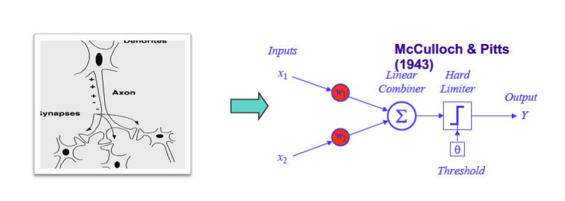
McCulloch & Pitt’s Neuron Model (1943)
Warren McCulloch and Walter Pitts created the first computational model of a neuron. The goal is to sum up the inputs and apply a threshold function. Their model used threshold-based activation with weights of $+1$ or $-1$, but did not support continuous weighting.
From Biological Neuron to Artificial Neuron
The McCulloch & Pitts neuron with threshold and binary weights can represent “AND”, “OR”, and “NOT” operations, but cannot represent “XOR”.
3. Rosenblatt’s Perceptron
Core Concept
Frank Rosenblatt introduced a learning rule for the computational neuron model in 1957. The perceptron generalizes McCulloch-Pitts neurons by introducing continuous weighting and using an activation function (typically a threshold function for the classic Rosenblatt perceptron).

Perceptron Learning Algorithm
The perceptron can find a decision boundary if classes are linearly separable. Given a dataset $D = {(x^{[1]}, y^{[1]}), \ldots, (x^{[N]}, y^{[N]})}$, the algorithm proceeds as follows:
- Initialize $w := 0_m$ (assume weight includes bias)
- For every training epoch:
- For every $(x^{[i]}, y^{[i]}) \in D$:
- $\hat{y}^{[i]} := \sigma(x^{[i]T} w)$ (only 0 or 1)
- $\text{err} := (y^{[i]} - \hat{y}^{[i]})$ (only $-1$, $0$, or $1$)
- $w := w + \text{err} \times x^{[i]}$
- For every $(x^{[i]}, y^{[i]}) \in D$:
Geometric Intuition
The decision boundary is a hyperplane in input space, and the weight vector $w$ is perpendicular to this decision boundary. Learning adjusts the orientation of the decision boundary.
Perceptron Limitations
The perceptron has several important limitations. As a linear classifier, it cannot learn non-linear boundaries and is limited to binary classification, making it unable to solve XOR problems. It does not converge if classes are not linearly separable. While many solutions may achieve zero training error, most will not be optimal in terms of generalization performance.
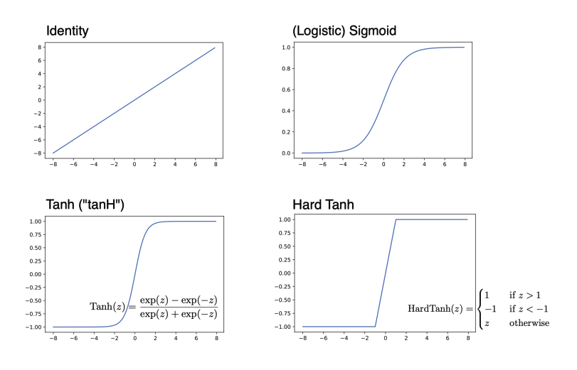
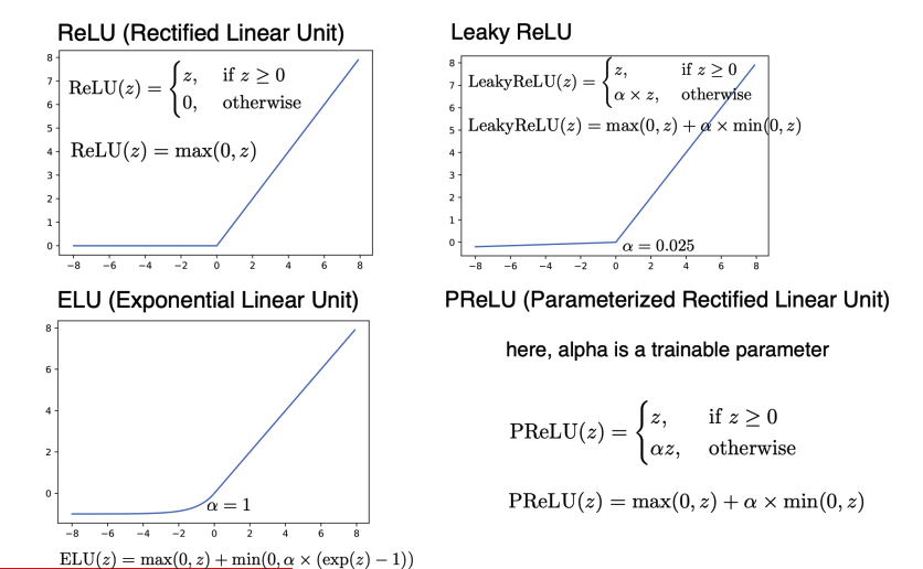
Activation Functions
Modern neural networks use various activation functions beyond the threshold function:
Sigmoid: Smooth and differentiable, outputs in $(0, 1)$
Tanh: Mean-centered, outputs in $(-1, 1)$. Advantages include mean centering, positive and negative values, and larger gradients. It’s important to normalize inputs to mean zero and use random weight initialization with average weight centered at zero.
ReLU: $\text{ReLU}(z) = \max(0, z)$
Leaky ReLU: Allows small negative values
ELU: Exponential Linear Unit
SELU: Scaled Exponential Linear Unit
4. Logistic Regression
Logistic Regression Neuron
For binary classes $y \in {0, 1}$, logistic regression uses a sigmoid activation function.
Probability Formulation
| Given the output $a = \sigma(w^T x)$, we compute the probability as $P(y = 1 | x) = a$, following the Bernoulli distribution. |
Maximum Likelihood Estimation
Under maximum likelihood estimation, we maximize the multi-sample likelihood:
\[L(w) = \prod_{i=1}^n P(y^{(i)}|x^{(i)})\]The log-likelihood is:
\[\log L(w) = \sum_{i=1}^n \log P(y^{(i)}|x^{(i)})\]Gradient Descent Learning Rule
We optimize via gradient descent using stochastic updates:
\[w := w + \eta \nabla_w \log P(y^{(i)}|x^{(i)})\]5. Multilayer Perceptron
Architecture
A multilayer perceptron is a computation graph with multiple fully-connected layers. By stacking multiple layers of perceptrons, the network can learn non-linear decision boundaries.
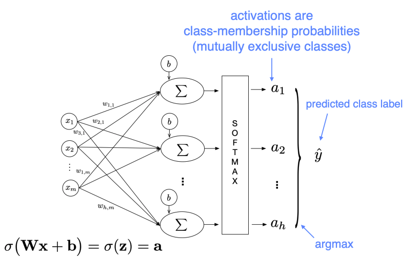
Multinomial (“Softmax”) Logistic Regression
For multi-class classification, we use the softmax function, which is a “soft” (differentiable) version of “max”:
Loss Function
Assuming one-hot encoding, the cross-entropy loss is:
\[L = -\sum_i y_i \log(\hat{y}_i)\]Solving XOR
Multilayer perceptrons can solve the XOR problem that single-layer perceptrons cannot. A single hidden layer is sufficient for the XOR problem, demonstrating the power of depth.
6. Backpropagation: An Algorithm to Train Models with Hidden Variables
The Training Problem
How can we train a multilayer model when there are no targets or ground truth for the hidden nodes? The solution is backpropagation.
Core Concept
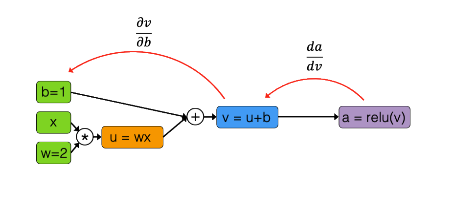
Neural networks are function compositions that can be represented as computation graphs. By applying the chain rule and working in reverse order, we can compute gradients efficiently:
\[\frac{\partial f}{\partial x_i} = \sum_j \frac{\partial f}{\partial z_j} \frac{\partial z_j}{\partial x_i}\]Computation Graphs
Computation graphs consist of input variables, intermediate computations, and outputs. The chain rule is applied in reverse to propagate gradients.
Forward pass: Compute activations from inputs to outputs
Backward pass: Compute gradients from outputs to inputs, where the local gradient is multiplied by the upstream gradient
Weight-Sharing
When the same weights are used in multiple locations in the network, gradients are accumulated from all uses of those weights.
7. PyTorch: Automated Differentiation
PyTorch provides automated differentiation, making it easy to train neural networks through three main steps:
Step 1: Definition - Define model architecture, specifying layers and activation functions
Step 2: Creation - Instantiate the model, initialize optimizer and loss function
Step 3: Training - Perform forward pass to compute predictions, compute loss, perform backward pass to compute gradients using .backward(), update weights using the optimizer, and zero gradients before the next iteration
8. Improvements to Optimization
Non-Convex Loss
While linear regression, Adaline, logistic regression, and softmax regression have convex loss functions, deep neural networks typically have non-convex loss landscapes. In practice, we usually end up at different local minima if we repeat the training.
Minibatch Training
Minibatch learning is a form of stochastic gradient descent where each minibatch can be considered a sample drawn from the training set. This means the gradient is noisier, which can be good (providing a chance to escape local minima) or bad (leading to extensive oscillation).
Learning Rate Decay
Due to batch effects, minibatch loss and gradients are approximations, typically resulting in oscillations. To dampen oscillations towards the end of training, we can decay the learning rate. However, decreasing the learning rate too early is dangerous. A practical tip is to try training the model without learning rate decay first, then add it later.
Common variants include:
- Exponential Decay: $\eta_t := \eta_0 e^{-k \cdot t}$ where $k$ is the decay rate
- Halving: $\eta_t := \eta_{t-1}/2$ where $t$ is a multiple of $T_0$ (e.g., $T_0 = 100$)
- Inverse decay: $\eta_t := \frac{\eta_0}{1 + k \cdot t}$
Training with Momentum
The main idea is to dampen oscillations by using “velocity” (the speed of the “movement” from previous updates). Not only move in the opposite direction of the gradient, but also move in the weighted averaged direction of the last few updates:
\[v_t = \gamma v_{t-1} + \eta \nabla_w L\] \[w_t = w_{t-1} - v_t\]Nesterov Momentum
Nesterov momentum is an improvement that looks ahead before making the step. Since we already know where the momentum part will push us in this step, we calculate the new gradient with that update in mind.
Adaptive Learning Rates
The rule of thumb for adaptive learning rates is to decrease learning if the gradient changes its direction and increase learning if the gradient stays consistent.
RMSProp
RMSProp is an unpublished but very popular algorithm by Geoff Hinton, based on Rprop and very similar to AdaDelta. The main idea is to divide the learning rate by an exponentially decreasing moving average of the squared gradients (RMS stands for “Root Mean Squared”). This takes into account that gradients can vary widely in magnitude.
ADAM (Adaptive Moment Estimation)
ADAM is probably the most widely used optimization algorithm in deep learning. It combines momentum with RMSProp:
- Momentum-like term: $m_t = \beta_1 m_{t-1} + (1 - \beta_1) \nabla_w L$
- RMSProp term: $v_t = \beta_2 v_{t-1} + (1 - \beta_2) (\nabla_w L)^2$
- ADAM update: $w_t = w_{t-1} - \frac{\eta}{\sqrt{v_t} + \epsilon} m_t$
9. Regularization
Where We Are
Good news: We can solve non-linear problems! Bad news: Our multilayer neural networks have lots of parameters and it’s easy to overfit the data.
Parameters vs Hyperparameters
Parameters (learned from data): weights (weight parameters) and biases (bias units)
Hyperparameters (set before training): minibatch size, data normalization schemes, number of epochs, number of hidden layers, number of hidden units, learning rates, loss function, activation function types, regularization schemes, weight initialization schemes, and optimization algorithm type
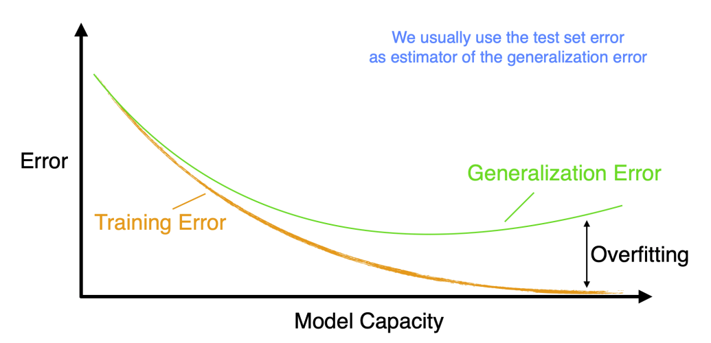
Overfitting and Underfitting
Underfitting occurs when the model is too simple, resulting in high bias. Overfitting occurs when the model is too complex, resulting in high variance. The goal is to find the right balance.
Bias-Variance Decomposition
\[\text{Total Error} = \text{Bias}^2 + \text{Variance} + \text{Irreducible Error}\]Bias is the error from incorrect assumptions, while variance is the error from sensitivity to the training set.
General Strategies to Avoid Overfitting
Collecting more data, especially high-quality data, is best and always recommended. Alternative approaches include semi-supervised learning, transfer learning, and self-supervised learning. Data augmentation is helpful, and reducing model capacity can also help.
Data Augmentation
The key idea is that if we know the label shouldn’t depend on a transformation $h(x)$, then we can generate new training data $(h(x^{(i)}), y^{(i)})$. However, we must already know something that our outcome doesn’t depend on. For image classification, this includes transformations like rotation, zooming, and sepia filters.
Reduce Network’s Capacity
The key idea is that the simplest model that matches the outputs should generalize the best. Strategies include choosing a smaller architecture (fewer hidden layers and units), adding dropout, using ReLU with L1 penalty to prune dead activations, enforcing smaller weights through early stopping or L2 norm penalty, and adding noise through dropout. With recent large language models and foundation models, it’s possible to use a large pretrained model and perform efficient fine-tuning.
Early Stopping
Split your dataset into three parts, using the test set only once at the end and using validation accuracy for tuning. Stop training early by observing the training/validation accuracy gap during training and stopping when the train and validation gap grows.
L2 Regularization
Add a penalty term to the loss function:
\[L_{\text{total}} = L_{\text{data}} + \lambda \sum_i w_i^2\]This encourages smaller weights and helps prevent overfitting. In PyTorch, use the weight_decay parameter in the optimizer.
Dropout
Randomly “drop” (set to zero) activations during training. Each neuron has probability $p$ of being dropped. This forces the network to learn redundant representations and acts as an ensemble of many networks. At test time, use all neurons but scale activations by $p$.
10. Normalization
Normalization and Gradient Descent
Normalizing inputs helps gradient descent converge faster by making the optimization landscape more isotropic (circular rather than elliptical).
Problem in Deep Models
Normalizing the inputs only affects the first hidden layer. What about the rest of the layers? Internal covariate shift refers to the problem that the distribution of layer inputs changes during training.
Batch Normalization (“BatchNorm”)
Batch normalization normalizes hidden layer inputs, helps with exploding/vanishing gradient problems, and can increase training stability and convergence rate. It can be understood as additional normalization layers with additional parameters.
Step 1: Normalize Net Inputs
For each minibatch, compute mean and variance, then normalize:
\[\hat{z} = \frac{z - \mu_{\text{batch}}}{\sqrt{\sigma^2_{\text{batch}} + \epsilon}}\]Step 2: Pre-Activation Scaling
Scale and shift:
\[\tilde{z} = \gamma \hat{z} + \beta\]where $\gamma$ and $\beta$ are learnable parameters. Technically, a BatchNorm layer could learn to perform standardization with zero mean and unit variance.
BatchNorm and Backpropagation
Gradients flow through normalization, with the chain rule applied to compute gradients with respect to $\gamma$, $\beta$, and inputs.
BatchNorm in PyTorch
Use nn.BatchNorm1d(num_features) for fully-connected layers and nn.BatchNorm2d(num_channels) for convolutional layers.
BatchNorm at Test-Time
Use an exponentially weighted average (moving average) of mean and variance:
running_mean = momentum * running_mean + (1 - momentum) * sample_mean
where momentum is typically around 0.1 (and the same for variance). Alternatively, you can also use global training set mean and variance.
Layer Normalization
Batch normalization calculates mean and standard deviation based on a minibatch, whereas layer normalization calculates mean and standard deviation based on feature/embedding vectors. In statistical language, batch normalization achieves zero mean unit variance, whereas layer normalization projects the feature vector to the unit sphere. Layer normalization is used in Transformers.
Initialization
Weight Initialization
We can’t initialize all weights to 0 due to the symmetry problem, but we want weights to be relatively small. Traditionally, we can initialize weights by sampling from a random uniform distribution in range $[0, 1]$, or better, $[-0.5, 0.5]$. Alternatively, we could sample from a Gaussian distribution with mean 0 and small variance (e.g., 0.1 or 0.01).
Xavier Initialization
Xavier Glorot and Yoshua Bengio introduced this method in their 2010 paper “Understanding the difficulty of training deep feedforward neural networks.” The method involves:
- Initializing weights from a Gaussian or uniform distribution
- Scaling the weights proportional to the number of inputs to the layer (for the first hidden layer, that is the number of features in the dataset; for the second hidden layer, that is the number of units in the first hidden layer)
Formula:
\[W \sim \mathcal{N}\left(0, \frac{2}{n_{\text{in}} + n_{\text{out}}}\right)\]He Initialization
Kaiming He et al. introduced this method in their 2015 paper “Delving deep into rectifiers: Surpassing human-level performance on imagenet classification.” Assuming activations with mean 0, Xavier initialization assumes a derivative of 1 for the activation function (which is reasonable for tanh). For ReLU, the activations are not centered at zero. He initialization takes this into account by adding a scaling factor of $\sqrt{2}$:
\[W \sim \mathcal{N}\left(0, \frac{2}{n_{\text{in}}}\right)\]Convolutional Neural Networks
Why Images Are Hard
Images present several challenges: high dimensionality (even small images have thousands of pixels), spatial structure (nearby pixels are correlated), and translation invariance (objects can appear anywhere in the image).
Full Connectivity Problem
Full connectivity is problematic for large inputs. For example, $3 \times 200 \times 200$ images imply 120,000 weights per neuron in the first hidden layer. This leads to too many parameters (causing overfitting) and is computationally expensive.
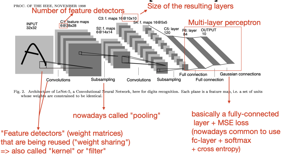
CNNs
Yann LeCun introduced convolutional neural networks in 1989. The key idea is to share parameters: instead of learning position-specific weights, learn weights defined for relative positions. Learn “filters” that are reused across the image to generalize across spatial translation of input. The core concept is to replace matrix multiplication in neural networks with a convolution. Later developments have shown that this approach can work for any graph-structured data, not just images.
Weight Sharing in Kernels
Reused weights are small and the same filter is applied to different regions of the input, dramatically reducing the number of parameters.
Pooling: Lossy Compression
Pooling reduces spatial dimensions. Max pooling takes the maximum value in each region, while average pooling takes the average value. Pooling provides translation invariance and reduces computation in subsequent layers.
Main Ideas of CNNs
Sparse-connectivity: A single element in the feature map is connected to only a small patch of pixels (very different from connecting to the whole input image in multilayer perceptrons)
Parameter-sharing: The same weights are used for different patches of the input image
Many layers: Combining extracted local patterns to global patterns
Key Concepts
Sparse Connectivity: Each neuron only connects to a small region of the input, reducing the number of parameters and exploiting local spatial structure.
Receptive Fields: The region of the input that affects a particular neuron. Receptive fields grow over depth, allowing deeper layers to represent more global features.
Parameter Sharing: Same filter weights used across the entire image, enabling detection of features regardless of position and dramatically reducing parameter count.
Impact of Convolutions on Size
Output size depends on input size, kernel size, stride, and padding:
\[\text{output size} = \left\lfloor \frac{\text{input size} - \text{kernel size} + 2 \times \text{padding}}{\text{stride}} \right\rfloor + 1\]Padding
Add zeros around the border of the input to preserve spatial dimensions. “Valid” padding means no padding, while “Same” padding ensures output size equals input size.
Backpropagation in CNNs
The same concept applies as before: multivariable chain rule, now with an additional weight-sharing constraint. Gradients are accumulated across all positions where a filter is applied. Convolution in the forward pass corresponds to transposed convolution in the backward pass.
Summary
We’ve covered the fundamentals of deep learning from perceptrons to CNNs. Key concepts include backpropagation, optimization, regularization, and normalization. Modern deep learning combines all these techniques. Next topics will cover more advanced architectures and generative models.