Lecture 15

A Linear Intro to Generative Models

Today’s Topics:

• 1. Generative Models
• 2. Generative and Discriminative Models
• 3. Example Discriminative Model:Logistic Regression
• 4. Example Generative Model:Naive Bayes
• 5. Discriminative vs Generative Models
• 6. Logistic Regression vs Naive Bayes
• 7. Modern DGMs

---

1.Generative Models

Deep Generative Models (DGM)

Key Characteristics

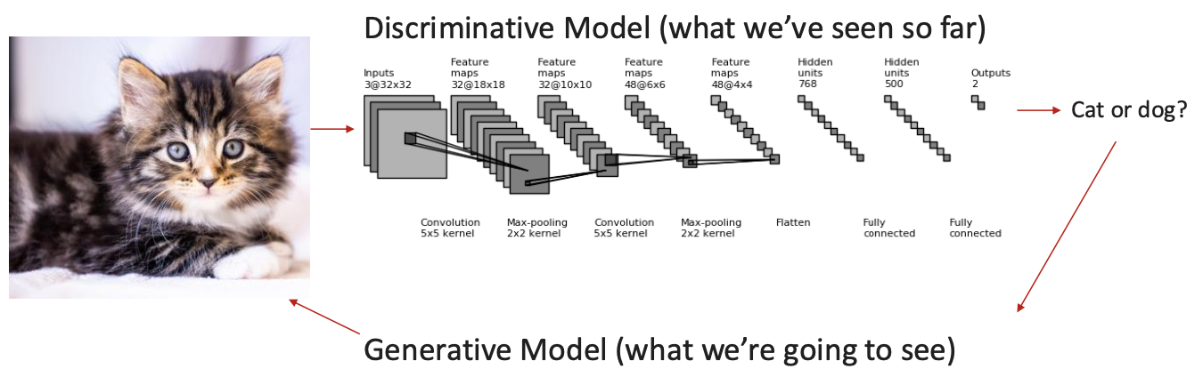
• Previoulsy, we learned about discriminative model that can classify images (e.g., CNN).
• Now, we will learn generative models that not only classify images, but they can also generate them on their own - such as ChatGPT, Gemini or DeepSeek.

Figure 1. Difference between discriminative and generative model

---

2. Generative and Discriminative Models

More detail about difference between two Models

1. Generative Models

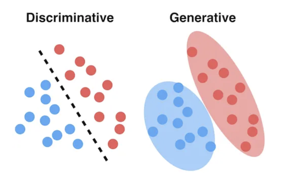
• Models focus on learning the underlying distribution of the data
• aim to understand how the data is generated, so allows them to create new data
• Models the joint distribution $P(X,Y)$ where $X$ represents the features Y denotes the class labels

2. Descriminative Models

• Models focus on modeling and decision boundary between classes
• learn conditional distribution $P(Y \mid X)$ which represents the probability of a class label given the input features
• used for classification tasks or distinguishing between classes based on features

Figure 2. entire data distribution vs conditional probability

---

3. Two paths to P(Y|X)

Descriminative Models

• Direct path
• When you observe X, Y then you directly learn $P(Y \mid X)$ which is the boundary between classes
• $P(Y \mid X)$ is, “Given X(data), what is the most likely Y(label)
• In classification, $\hat{Y} = argmax_Y P(Y \mid X)$

Generative Models

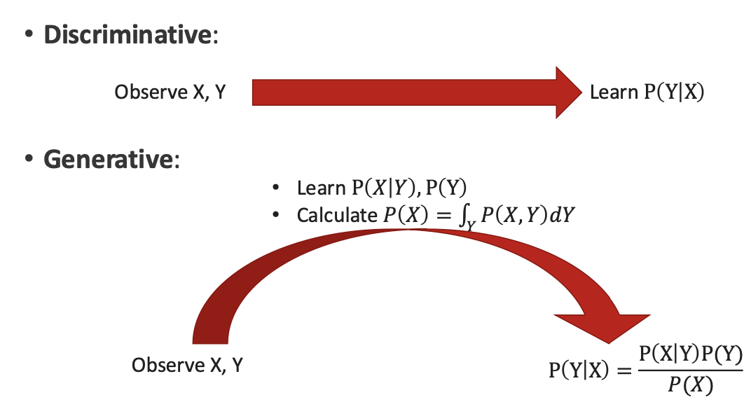
• Observe (X, Y)
• you first learn:
  • $P(X \mid Y)$ → how data X is distributed within each class
  • $P(Y)$ → Distribution of Y (the prior)
• also you can calculate $P(X) = \int_{Y} P(X,Y) \ dY$ which is the marginal probability of X regardless of Y
• finally we yield $P(Y \mid X)$ using bayes’ rule
  • $P(Y \mid X) = \frac{P(X \mid Y) \, P(Y)}{P(X)}$
• In classification task, we don’t need to calculate $P(X)$
  • $\hat{Y} = argmax_Y P(X \mid Y) \ P(Y)$

Figure 3. Path to P(Y|X)

---

3. Example Discriminative Model:Logistic Regression

Core Characteristic of Discriminative Model: Parameterization

• Parameterization in Logistic Regression
  • $P(Y = 1 \mid X) = \sigma(\theta^{T} \ X)$, where $\sigma(z) = \frac{1}{1+e^{-z}}$ is the sigmoid function
  • $P(Y = 0 \mid X) = 1 - P(Y=1 \mid X)$
  • “Why do we choose this form of parameterization?”
  • Because in logistic regression, we assume the log-odds of the probability is a linear function of the input

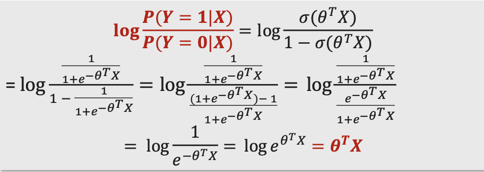
• In logistic regression the log odds is a linear combination of the features X
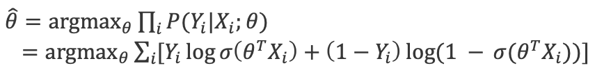
• Estimate $\hat{\theta}$ form observation:

---

4. Example Generative Model: Naive Bayes

Core Characteristic of Generative Model:

We observe X and Y. Then we learn $P(X \mid Y) and P(Y)$ and we use it to derive $P(Y \mid X) = \frac{P(X \mid Y) P(Y)}{P(X)}$, where $P(Y = 1) = \frac{number \hspace{1em} of \hspace{1em} samples \hspace{1em} with \hspace{1em} Y = K}{Total \hspace{1em} samples}$

• Parameterize
  • Assume $P(X \mid Y) = \prod_{j=1}^{d} P(X_j \mid Y)$
  • $P(X_j \mid Y) = N (\mu_{jk} , \sigma_{jk}^{2})$
• Estimate
  • $\hat{\mu} , \hat{\sigma} = argmax_{\mu , \sigma} P(X \mid Y)$
• Calculate
  • $P(Y=1 \mid X) = \frac{\prod_{j=1}^{d} P(X_j \mid Y) P(Y=1)}{P(X)}$

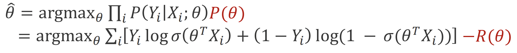
MAP / Regularization Note:

Logistic regression: We change our $\hat{\theta}$ estimates from observations by:

---

5. Discriminative vs Generative Models

• Discriminative models optimize the conditional likelihood: $\hat{\theta_{disc}} = argmax_{\theta} P(Y \mid X; \theta) = argmax_{\theta} \frac{P(X \mid Y ; \theta) P(Y; \theta)}{P(X; \theta)}$

• Generative models optimize the joint likelihood: $\hat{\theta_{disc}} = argmax_{\theta} P(X, Y; \theta) = argmax_{\theta} P(X \mid Y ; \theta) P(Y; \theta)$

  This means they are exactly the same optimization when $P(X; \theta)$ is invariant to $\theta$

---

6. Logistic Regression vs Naive Bayes

Logistic Regression**

• Type : Discriminative
• It directly models the decision boundary: $P(Y \mid X; \theta)$
• It does not models how data is generated only the probability that a given (X) belongs to a certain class (Y )
• Defines : $P(Y \mid X; \theta) = \sigma(\theta^T X) = \frac{1}{1 + e^{-\theta^T X}}$
• Estimates:
  • Parameters are learned by maximizing the conditional likelihood: $\hat{\theta_{lr}} = argmax_{\theta} P(Y \mid X; \theta)$
  • Or equivalently, by maximizing the log-likelihood: $\hat{\theta_{lr}} = \arg\max_{\theta} \sum_i \left[Y_i \log \sigma(\theta^{T} X_i) + (1 - Y_i) \log \left(1 - \sigma(\theta^{T} X_i)\right)\right]$
• Properties:
  • Lower asymptotic error : As the sample size approaches infinity, the learned boundary becomes optimal and the error rate decreases.
  • Slower convergence : Requires more data to achieve stable performance because it learns only from discriminative information.

---

Naive Bayes

• Type : Generative
  • Learns the joint distribution of data $P(X, Y; \theta) = P(Y; \theta) \cdot P(X \mid Y; \theta)$
  • Using Bayes’ rule, we can derive the posterior: $P(Y \mid X) = \frac{P(X \mid Y) \, P(Y)}{P(X)}$
• Assumption: Conditional independence assumption $P(X \mid Y) = \prod_{j=1}^{d} P(X_j \mid Y)$
• Estimates: Parameters are learned by maximizing the joint likelihood: $\hat{\theta_{NB}} = \arg\max_{\theta} P(X, Y; \theta)$
• Properties:
  • Higher asymptotic error : Because the independence assumption is not always true, it can produce biased estimates when data features are correlated
  • Faster convergence : Simpler assumptions mean fewer parameters, allowing it to learn well even from small datasets

---

Discriminative vs Generative: A proposition

• “While discriminative learning has lower asymptotic error, a generative classifier may also approach its (higher) asymptotic error much faster.”
• This statement compares the learning efficiency and error behavior of discriminative vs generative models
• Underlying Assumption :
  • Generative models of the form $P(X, Y; \theta)$ make more simplifying assumptions than discriminative models of the form $P(Y \mid X; \theta)$
  • These assumptions often allow faster convergence (fewer samples needed), but may lead to higher asymptotic error due to bias in modeling
  • However, it is not always true In some data distributions, discriminative and generative approaches can perform similarly, or even the opposite may occur, depending on model misspecification

---

7. Modern Deep Generative Models (DGMs)

• Goal : To design generative models of the form $P(X, Y; \theta)$ that can model complex data distributions without making overly strong simplifying assumptions.
• Key Idea : Hidden Structure ( z ): Deep generative models introduce a latent (hidden) variable ( z ) that captures the underlying structure of high-dimensional observations ( x )
  • ( z ) explains or encodes meaningful patterns in the data
  • ( x ) is generated from ( z ) through a probabilistic process, e.g. $P_{\theta} (x \mid z)$
  • But we never directly observe the latent variable (z )
  • Because of this, two key computations become difficult:
    • 1. Marginal likelihood : $p_\theta(x) = \int p_\theta(x, z)\,dz$ We must integrate over all possible latent variables ( z ), which is intractable in high-dimensional space
    • 1. Posterior inference : $p_\theta(z \mid x) \propto p_\theta(x \mid z)\,p(z)$. The posterior distribution of ( z ) given ( x ) is typically complex and cannot be computed analytically.
    • 1. Each type of Deep Generative Model (DGM) makes a tradeoff between: Expressiveness (how flexible the model is) and Computational tractability (how easy it is to compute or train)