Lecture 17

Generative Adversarial Networks (GANs)

November 3 — Generative Adversarial Networks (GANs)

Topics

Review: Autoencoders
Generative Adversarial Networks (GANs)
GANs and VAEs: A Unified View

1. Autoencoders (Review)

Goal: Learn a compressed latent representation of input ( x ).

Structure: $ \hat{x} = f(h) = f(g(x)) $ where:

( $g$ ): encoder
( $f$ ): decoder

Variants

Denoising Autoencoders

Add noise (e.g., dropout or Gaussian noise) to input.
Train to reconstruct the original, uncorrupted input.
Purpose: Learn robust representations that can remove noise.

Autoencoders with Dropout

Dropout layers encourage redundancy in learned features.
Improves generalization and robustness to missing inputs.

Sparse Autoencoders

Loss function: $ L = \lVert x - \hat{x} \rVert^2 + \lambda \sum_i |h_i| $
Adds an L1 penalty on activations to enforce sparsity.
Produces interpretable features — each neuron learns a distinct factor.

Variational Autoencoders (VAEs)

Latent variable ( $z \sim \mathcal{N}(0, I)$ )
Enables sampling new data points.
Provides a probabilistic framework for generative modeling.
Objective: maximize the evidence lower bound (ELBO)

2. Generative Adversarial Networks (GANs)

Overview

Generative Adversarial Networks (GANs) were introduced by Goodfellow et al. (2014), and is a generative modeling framework between a generator that produces synthetic samples and a discriminator that tries to distinguish them from real data. Unlike autoencoders or autoregressive models, GANs can generate an entire sample with less steps.

Motivation

Traditional generative models (Gussian Mixtures, VAEs, and autoencoders) often struggle to uncover the complexity of high-dimensional data like that of images. GANs are flexible and capable of learning implicit data distributions. This makes them useful for image synthesis, style transfer, and text to image applications like those developed by OpenAI (DALL-E 2) and Google (Imagen).

Architecture and Training

Generator ($G_\theta$)

Maps a noise vector $z \sim p(z)$ (often Normal(0, I)) to a data-space sample $x = G_\theta(z)$.
Goal: produce samples indistinguishable from real data $x \sim p_{data}$.
Fool the discriminator (increase $D(G(z))$)
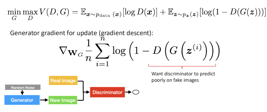
Trained via gradient descent to minimize $-\log D(G(z))$.

Gradient Descent with GAN — **Figure 1.** The adversarial training loop between generator and discriminator.

Discriminator ($D_\phi$)

Binary classifier outputting $D_\phi(x)\in(0,1)$, interpreted as $P(\text{real}\mid x)$.
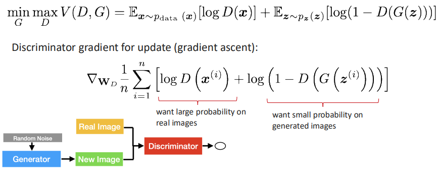
Trained to assign high probability to real data and low probability to generated data.
Discriminator loss (binary cross-entropy form):

\[\mathcal{L}_D = -\mathbb{E}_{x\sim p_{\text{data}}}[\log D_\phi(x)] - \mathbb{E}_{z\sim p(z)}[\log(1-D_\phi(G_\theta(z)))]\]

Updated by gradient descent on $\mathcal{L}_D$.

Gradient Ascent with GAN — **Figure 1.** The adversarial training loop between generator and discriminator.

Minimax Objective

“max” and “min” Objective

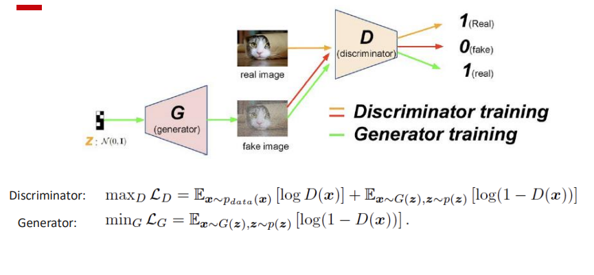
The discriminator outputs a probability $D_\phi(x)\in(0,1)$ interpreted as $P(\text{real}\mid x)$. The GAN game is:

\[\min_\theta \max_\phi \; \mathbb{E}_{x\sim p_{\text{data}}}[\log D_\phi(x)] + \mathbb{E}_{z\sim p(z)}[\log(1-D_\phi(G_\theta(z)))]\]

Discriminator step ($\max_\phi$): increase $\log D_\phi(x)$ for real $x$ and increase $\log(1-D_\phi(G_\theta(z)))$ for fake samples. This pushes $D(x)\to 1$ and $D(G(z))\to 0$.
Generator step ($\min_\theta$): make generated samples look real, i.e., push $D(G(z))$ upward (toward 1). In practice, we use the non-saturating generator loss for stronger gradients:

\[\mathcal{L}_G = -\mathbb{E}_{z\sim p(z)}[\log D_\phi(G_\theta(z))]\]

The generator minimizes this value by making its outputs hard to distinguish, while the discriminator maximizes it by improving classification.

Discriminator vs. Generator Training — **Figure 1.** The adversarial training loop between generator and discriminator.

Training Characteristics

Training alternates between both networks. Convergence ideally occurs at Nash Equilibrium, where the generator’s distribution equals the true data distribution and the discriminator outputs 0.5 for all inputs.

In practice training is often unstable:

Oscillatory losses between G and D
Mode collapse (one prototype sample repeated)
Vanishing gradients if D dominates this can lead to non-saturating loss being recommended
Hyperparameter sensitivity (learning rate, architecture, batch size)
If the discriminator is too strong, gradients for $G$ vanish and training stalls.
If the discriminator is too weak, $G$ can exploit $D$ and generate unrealistic samples that still fool it.

Interpretations and Variants

A pure equilibrium may not exist, which explains observed oscillations and non-convergence.

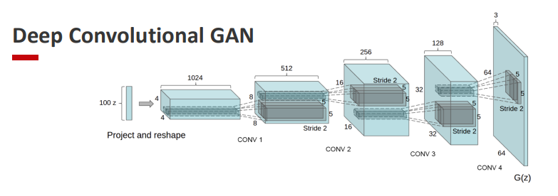
Deep Convolutional GAN (DC-GAN)

Introduces convolutional architectures to stabilize training and capture spatial features.

3. GANs and VAEs: A Unified View

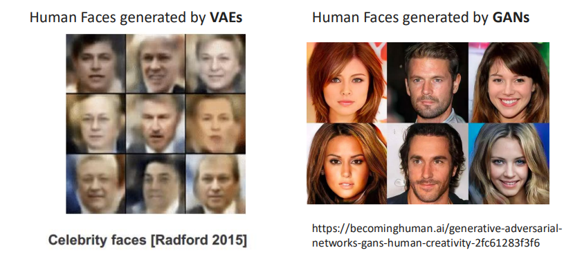
GAN is minimizing the KL divergence between $P_{\theta}$ and $Q$. On the other hand, the VAE is minimizing the KL divergence between $Q$ and $P_{\theta}$. GANs tend to miss the mode, whereas VAEs tend to cover regions with small values of $p_{data}$.

A Unified View

Feature	Autoencoders (AEs)	Variational Autoencoders (VAEs)	GANs
Goal	Learn latent representations	Probabilistic generative model	Adversarial generative model
Latent Variable	Deterministic ( $h = g(x)$ )	( $z \sim \mathcal{N}(0, I)$ )	( $z \sim p_z(z)$ )
Training	Reconstruction loss	ELBO (KL + reconstruction)	Adversarial minimax loss
Sampling	Deterministic decode	Random sampling via latent prior	Generator sampling ( G(z) )
Weakness	Not generative	Blurry outputs	Instability in training

VAEs vs. GANs: a cloesup

Aspect	Variational Autoencoder (VAE)	Generative Adversarial Network (GAN)
Objective	Single ELBO maximization	Two opposing objectives ($\min_G$, $\max_D$)
Regularization	KL term via prior $p(z)$	Implicit regularization via adversarial feedback
Inference Model	$q_\phi(z \mid x)$	$p_\theta(x \mid y)$, $q_\phi(y \mid x)$
Generation	Explicit probability model	Implicit distribution (no likelihood)

GAN vs. VAE — **Figure 1.** The adversarial training loop between generator and discriminator.

GANs can be expressed in a variational-EM-like framework:

E-step: update discriminator to approximate $q_\phi(y \mid x)$
M-step: update generator to improve $p_\theta(x \mid y)$

Common Problems

Problem	Explanation	Typical Fixes
Mode Collapse	Generator outputs few modes of data	Mini-batch discrimination, WGAN, feature matching
Vanishing Gradient	Discriminator too strong	Non-saturating loss (maximize $\log D(G(z))$)
Training Oscillation	No stable equilibrium	Gradient penalty, slow updates, learning-rate tuning
Over-fit Discriminator	Memorizes training data	Dropout, label smoothing

Empirically, GANs generalize only when the discriminator capacity and training data are balanced.
Otherwise, Jensen–Shannon and Wasserstein divergence analyses can be misleading in finite settings.

References

Goodfellow et al. (2014) Generative Adversarial Nets (NIPS).
Arora & Hardt (2017) Generative Adversarial Networks: Some Open Questions (OffConvex Blog).
Radford et al. (2015) Unsupervised Representation Learning with Deep Convolutional GANs.
Hu et al. (2017) Unifying Deep Generative Models.