Lecture 19
Sequence Learning with RNNs
Motivation: Why Text Modeling Is Challenging
Modeling text sequences is difficult due to:
- Variable sequence length
- Long-range dependencies
- Need for generative models
- Large data requirements
Historical Approaches
Bag-of-Words (BOW)
Represents text as unordered word counts.
Problem: Word order is lost
Example:
- “NOT good”
- “good NOT”
become identical vectors.
Hidden Markov Models (HMMs)
Use the Markov assumption:
\[P(Y_n \mid X_1,\ldots,X_n) = P(Y_n \mid X_n)\]Problem: Only captures one-step dependencies.
Convolutional Neural Networks (CNNs)
Capture local patterns using filters.
Limitation: Require fixed-length input; cannot naturally handle long sequences.
Recurrent Neural Networks
RNNs address sequential dependence using recurrent connections.

The Recurrence Equation
\[h^{(t)} = \sigma(W_{hx}x^{(t)} + W_{hh}h^{(t-1)} + b_h)\]Where:
- $h^{(t)}$: Hidden state
- $x^{(t)}$: Input at time $t$
- $W_{hx}, W_{hh}$: Input and recurrent weights
- $\sigma$: Typically
tanh
Unrolling Through Time
Unrolling converts an RNN into a deep network with depth equal to sequence length.
RNN Architectures
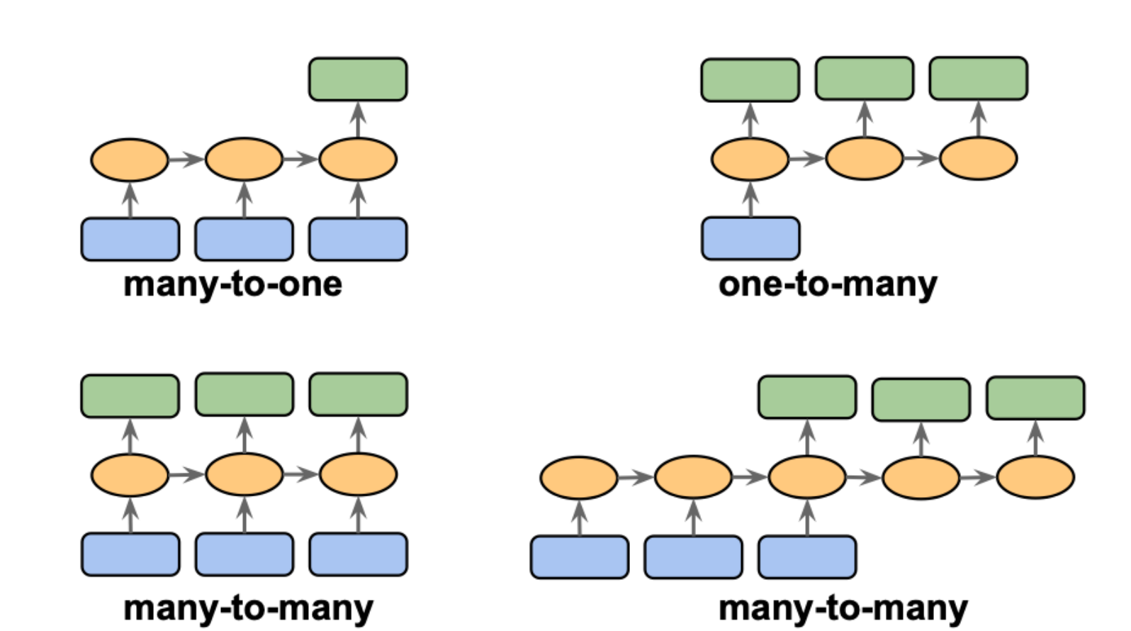
- Many-to-One: sentiment classification
- One-to-Many: image captioning
- Many-to-Many:
- synchronous: video captioning
- delayed: machine translation
Training RNNs: Backpropagation Through Time (BPTT)
Training RNNs involves unrolling through time and applying the chain rule.
Gradient Expression
\[\frac{\partial L^{(t)}}{\partial W_{hh}} = \frac{\partial L^{(t)}}{\partial y^{(t)}} \frac{\partial y^{(t)}}{\partial h^{(t)}} \Biggl( \sum_{k=1}^t \frac{\partial h^{(t)}}{\partial h^{(k)}} \frac{\partial h^{(k)}}{\partial W_{hh}} \Biggr)\]Key term:
\[\frac{\partial h^{(t)}}{\partial h^{(k)}} = \prod_{i=k+1}^{t} \frac{\partial h^{(i)}}{\partial h^{(i-1)}}\]A product of many Jacobians → unstable.
Vanishing and Exploding Gradients
- If Jacobians < 1 → vanishing gradients
- If Jacobians > 1 → exploding gradients
Consequences:
- Loss of long-range memory
- Training instability
Remedies
- Gradient clipping
- Truncated BPTT
- LSTM / GRU architectures
Long Short-Term Memory (LSTM)
LSTMs solve gradient issues by introducing a cell state $c_t$ that acts as a memory highway.
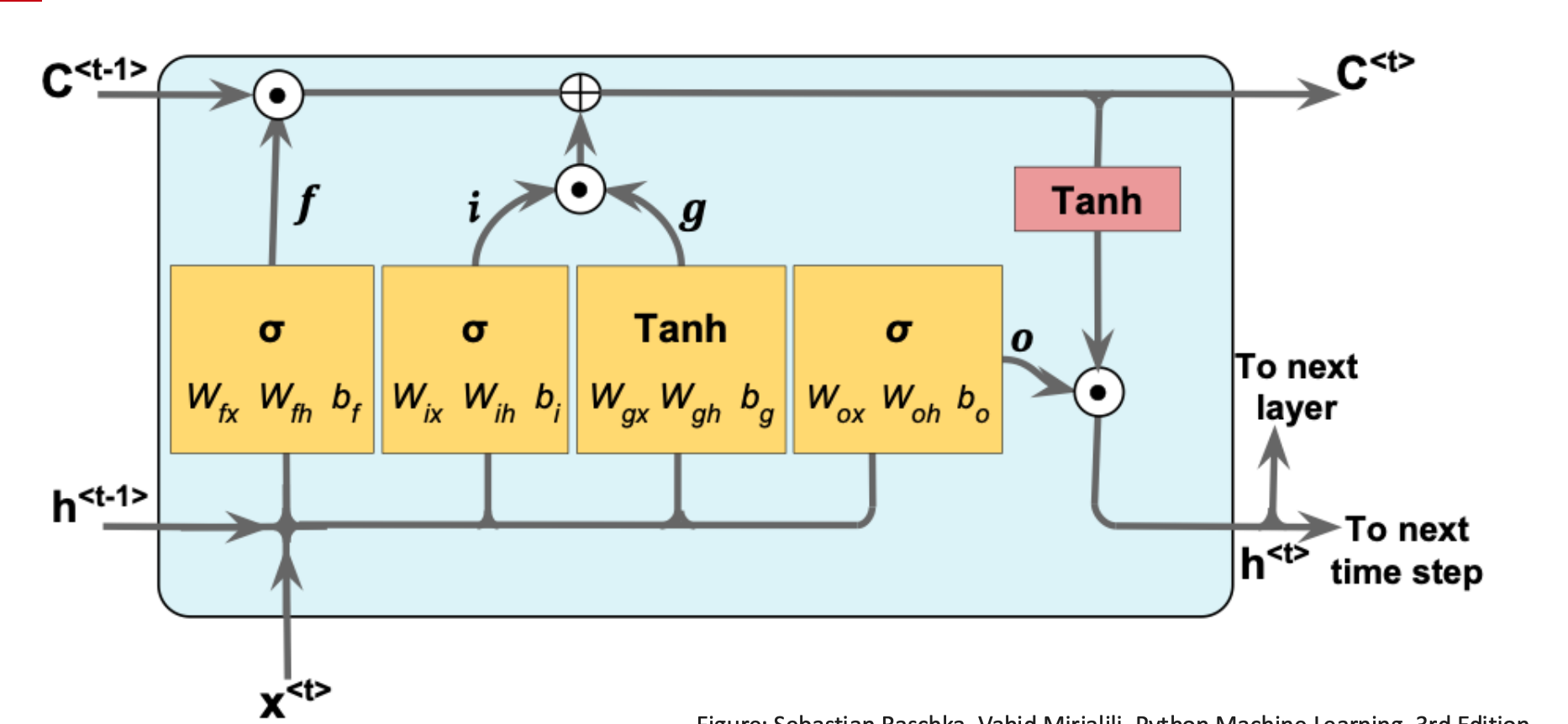
LSTM Gate Equations
\[\begin{aligned} f_t &= \sigma(W_f[x_t, h_{t-1}] + b_f) \\ i_t &= \sigma(W_i[x_t, h_{t-1}] + b_i) \\ g_t &= \tanh(W_g[x_t, h_{t-1}] + b_g) \\ c_t &= f_t \odot c_{t-1} + i_t \odot g_t \\ o_t &= \sigma(W_o[x_t, h_{t-1}] + b_o) \\ h_t &= o_t \odot \tanh(c_t) \end{aligned}\]Interpretation
- Forget gate: remove irrelevant memory
- Input gate + candidate: add new information
- Output gate: expose memory to next layer
- Cell state: preserves long-term gradients
Forget gate controls which information is remembered, and which is forgotten. It can reset the cell state:
\[f_{t} = \sigma(W_{fx} x^t + W_{fh} h^{t - 1} + b_{f})\]The sigmoid activation function has a range of $[0, 1]$. The output from the forget gate $f_{t}$ is later multiplied element-wise with the cell state. If $f_{t}$ is close to 0, it can make the cell state $C$ to “forget” some information.
Input gate adds stuff to the cell state:
\[i_{t} = \sigma(W_{ix} x^t + W_{ih} h^{t - 1} + b_{i})\]Input node
\[g_{t} =\tanh(W_{gx} x^t + W_{gh} h^{t-1} + b_{g})\]is element-wise multiplied with the input gate. The product then later is element-wise added to the cell state $C$.
Output gate is used to update the values of hidden units:
\[o_{t} = \sigma(W_{ox} x^t + W_{oh} h^{t-1} + b_{o}).\]The new value for the hidden unit will be the element-wise product between $\tanh(C^t)$ and $o_{t}$.
Why LSTMs help with vanishing gradients
A key reason LSTMs work better than vanilla RNNs is how the cell state (c_t) is updated. Recall the cell update:
\[c_t = f_t \odot c_{t-1} + i_t \odot g_t.\]If we look at the gradient of the loss (L) with respect to an earlier cell state (c_{t-k}), the dominant term is a product of forget gates:
\[\frac{\partial L}{\partial c_{t-k}} \approx \frac{\partial L}{\partial c_t} \prod_{j=t-k+1}^{t} f_j.\]- When the forget gates (f_j) are close to 1, the product stays close to 1 and gradients can flow back over many time steps.
- When the model decides some information is no longer needed, it can set (f_j) closer to 0, actively “forgetting” that part of the state.
This is very different from a vanilla RNN, where the hidden state is repeatedly multiplied by a weight matrix and passed through a nonlinearity. In that case, the Jacobian often has eigenvalues much smaller (or larger) than 1, leading to vanishing or exploding gradients.
The LSTM cell therefore provides an almost linear highway for gradients along the (c_t) path, with the gates controlling when to preserve information and when to reset it.
Preparing Text for RNNs
Step 1 — Build Vocabulary
Include: <unk>, <pad>, <bos>, <eos>.
Step 2 — Convert Text to Indices
Pad sequences to equal length for batching.
Step 3 — One-Hot Encoding (conceptual)
Not used in modern practice due to high dimensionality.
Step 4 — Word Embeddings
Learned dense vectors:
- Low dimension (e.g., 300-D)
- Similar words → similar embeddings
- Implemented via
nn.Embedding
RNNs for Generative Modeling
RNNs model the autoregressive distribution:
$P_{\theta}(X) = \prod_{t} P_{\theta}(X_t \mid X_{<t})$
Training objective:
$\max_{\theta} \sum_i \sum_t \log P_{\theta}(X_{i,t} \mid X_{i,<t})$
Used in classic language modeling.
Many-to-One Word RNN Example
- Build vocabulary
- Convert text → indices
- Convert indices → embeddings
- Feed sequence into RNN
- Use final hidden state for classification
Summary
| Concept | Description |
|---|---|
| RNN | Maintains hidden state to model sequential data |
| BPTT | Unrolls through time; gradient instability |
| LSTM | Gates + memory cell enable long-term learning |
| Gradient Clipping | Prevents gradient explosion |
| Truncated BPTT | Limits backpropagation depth |
| Embeddings | Dense word representations |
| Applications | NLP, speech, translation, time series |