Lecture 20

Attention and Transformers

Attention and Transformer Architecture

The Attention Mechanism

Motivation: Different parts of our input relate to different parts of our output. Sometimes these important relationships can be far apart, like in machine translation. Attention helps us dynamically calculate what is important.

Why Attention Was Needed (Long-Range Dependency Problem)

RNNs compress an entire input sequence into a single hidden vector, which makes capturing long-range dependencies difficult.
During backpropagation, gradients must pass through many time steps, causing vanishing/exploding gradients.

Attention solves this by directly referencing the entire input sequence when predicting each output, instead of relying on hidden states to store all information.

Key insight: Attention creates a constant path length between any two positions, unlike the sequential dependency in RNNs.

Origin: Originally from Natural Language Processing (NLP) and language translation.
Core Idea: Assign an attention weight to each word to signal how much we should “attend” to that word.
Evolution: We later learned that attention and recurrence are not both necessary, popularized by the paper “Attention is all you need”.

Hard Attention

Hard attention makes a binary 0/1 decision about where to attend. It asks: “Is this input important to this prediction or not?”

Pros: Easy to interpret.
Cons: Difficult to train; requires reinforcement learning. It is rarely used in practice.

Soft Attention

Rather than a binary decision, we assign a continuous weight between 0 and 1 for each input.

Mechanism: A softmax function is used to compute weights, ensuring they are real values between 0 and 1 and that the sum of all weights equals 1.
Interpretation: Each weight represents the proportion of influence that input has on the current prediction.
Visualization: in Machine Translation, visualizing the influence of inputs on outputs usually shows a strong diagonal (token-to-token), except where word order differs (e.g., French vs. English nouns).

Soft Attention vs. RNN for Image Captioning

RNNs:

Only look at the image (or the 1-D CNN embedding of the original image) once to try to find important features.
Successively refer back to the same hidden state, which must encode information about both foreground and background.

Soft Attention:

Generates an attention map, which refers back to a 2-D CNN embedding at each hidden state.
Generates a word and an input to the next hidden state.
Keeps looping back to the input, tying weights to a combination of learnable features. Allows each word in the caption to refer to different parts of the image.
The attention weights are computed as:

\[a_{i,j} = \mathrm{softmax}_j(x_i^\top x_j)\]

and the final attention output is:

\[A_i = \sum_j a_{i,j} x_j.\]

Aside: CNNs were an example of Hard Attention. As the filter slides over the image, the part of the image inside the filter gets attention weight 1, and the rest gets weight 0.

Why Attention Reduces the Need for Recurrence

Attention repeatedly refers back to the input, so the hidden state no longer needs to store all global information.
This insight led to eliminating recurrence entirely in the Transformer.

Self Attention

Motivation: Can we get rid of the sequential RNN component? Since attention already ties inputs across the sequence, is it necessary to continue to loop over it?

Basic Self Attention

Main procedure:

Derive Attention Weights: Calculate similarity between each current input and all other inputs.
Normalize: Use softmax to normalize weights.
Compute: Calculate attention from normalized weights and corresponding inputs.

Computing Weights: We use a dot product when computing attention weights. Dot products are similar to cosine similarity, but are sensitive to vector magnitudes. Since we will be learning weights (not in this basic version, but later), there is no need to normalize in practice.

The self-attention corresponding to the $i$ -th input, $x_i$ , is $A_i$ .
$A_i$ is the weighted sum over all inputs, where the weight for $x_j$ is $a_{i,j}$ .
$a_{i,j}$ is the softmax output for the dot product between $x_i$ and $x_j$ .

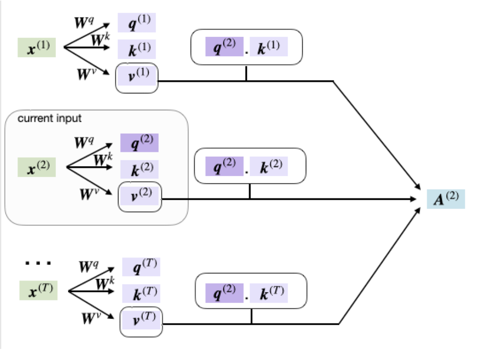
Learnable Self Attention

The basic version has no learnable parameters. To fix this, we add three trainable weight matrices to be multiplied by input sequence embeddings: Query, Key, and Value.

Query ( $Q$ ): Represents what the token is “asking” the rest of the sequence.
Key ( $K$ ): Describes how the token “advertises” the information it holds.
Value ( $V$ ): The actual content shared if other tokens pay attention to it.

The Process: For every token, the model compares its Query to the Keys of all tokens in the sequence.

High Alignment: If query/key align well $\rightarrow$ High attention score.
Low Alignment: If not $\rightarrow$ Low attention score.

These scores are normalized to act as weights. Each token builds a new representation by taking a weighted blend of the Value vectors from all tokens. Every position becomes a learned mixture of information pulled from everywhere else, with the mixing proportions determined by how relevant the model thinks each other token is.

Why this works: Because $Q$ , $K$ , and $V$ are trainable, the model learns its own notion of “relevant context.” Early layers may focus on nearby words; deeper layers may learn to link pronouns to nouns or relate the start/end of sentences. This structure emerges from adjusting those weight matrices to reduce training loss, turning self-attention into a flexible, learned mechanism for combining information across a sequence.

The Transformer

Originally proposed for machine translation. It consists of two stacks side-by-side, each replicated $N$ times.

Left Stack: Encoder (input stack), used in encoder–decoder models like translation.
Right Stack: Decoder (output stack). This is the only stack used in GPT-style models.
Encoder layers contain only self-attention.
Decoder layers contain both masked self-attention and cross-attention to the encoder output.

Components

Multi-headed Attention: Applies self-attention multiple times in parallel. $Q$ , $K$ , and $V$ matrices have multiple rows, allowing the model to attend to different parts of the sequence differently simultaneously.
Multi-head attention applies several attention heads in parallel:

\[\text{head}_h = \mathrm{Attention}(Q W_h^Q,\; K W_h^K,\; V W_h^V)\]

The final output concatenates all heads:

\[\text{MHA}(Q,K,V) = \text{Concat}(\text{head}_1,\dots,\text{head}_H)\, W^O.\]

Skip Connections (Residuals): We add Input + (Input passed through attention layer). This helps manage vanishing gradients.

Transformer Tricks (NLP)

Self-Attention: Each layer combines words with others.
Multi-headed Attention: 8 attention heads learned independently.
Normalized Dot-Product Attention: Removes bias in the dot product when using large networks.
Positional Encodings: Ensures that even without an RNN, the model can distinguish positions.
- Note: This may not matter as much as thought, as the attention mechanism can generate position-specific encodings itself.