Lecture 21: GPT Architectures
From RNNs to Transformers to GPT - Understanding the evolution of modern language models
Today’s Topics:
- Part 1: From RNN to Self-Attention & The Transformer
- Part 2: GPT Architecture & Probabilistic Model
- Part 3: The Evolution of the GPT Series (GPT-1 to GPT-4)
- Part 4: Mixture of Experts (MoE) & Final Summary
- Conclusion
- References
Part 1: From RNN to Self-Attention & The Transformer
(Ref: Slides 1–10, 15–16)
1. The Limitations of RNNs
(Ref: Slides 2–3)
Recurrent Neural Networks (RNNs) were the dominant architecture for sequence modeling before the Transformer era. RNNs process sequences sequentially, maintaining a hidden state $h^{\langle t \rangle}$ that gets updated at each time step:
While this recurrent structure allows the model to process sequences of arbitrary length, it introduces several critical problems:
-
Sequential Processing Bottleneck: Each token must be processed one at a time, meaning computation cannot be parallelized across the sequence. This makes training extremely slow for long sequences.
-
Long-Range Dependency Problem: Information from early tokens must be passed through many intermediate hidden states to reach later positions. Despite improvements like LSTMs and GRUs, gradients still tend to vanish or explode over long sequences, making it difficult to capture dependencies between distant tokens.
-
Fixed-Capacity Hidden State: The entire sequence history must be compressed into a single fixed-dimensional vector $h^{\langle t \rangle}$, creating an information bottleneck.
Key Insight: We need an architecture that:
- Enables parallel computation across sequence positions
- Allows direct connections between any pair of tokens
- Avoids compressing all information into a single bottleneck
This motivates the Transformer architecture.
2. The Transformer Solution
(Ref: Slides 4–5)
The Transformer, introduced by Vaswani et al. (2017) in “Attention Is All You Need,” replaces recurrence with attention mechanisms. Instead of sequentially processing tokens, the Transformer computes interactions between all pairs of positions in parallel using self-attention.
Key advantages:
- Parallelization: All token representations can be computed simultaneously
- Direct long-range connections: Every token can directly attend to every other token, eliminating the vanishing gradient problem for long-range dependencies
- Dynamic context: Each token’s representation is a weighted combination of all other tokens, with weights learned based on content similarity
The Transformer consists of:
- Encoder: Processes the input sequence with bidirectional attention
- Decoder: Generates the output sequence with masked (causal) attention and cross-attention to encoder outputs
 —
—
3. Self-Attention: The Basic (Non-Learnable) Form
Before introducing the learnable self-attention used in Transformers, let’s understand the simplest form of self-attention to grasp the core concept.
Given a sequence of token embeddings:
where $T$ is the sequence length and $d$ is the embedding dimension.
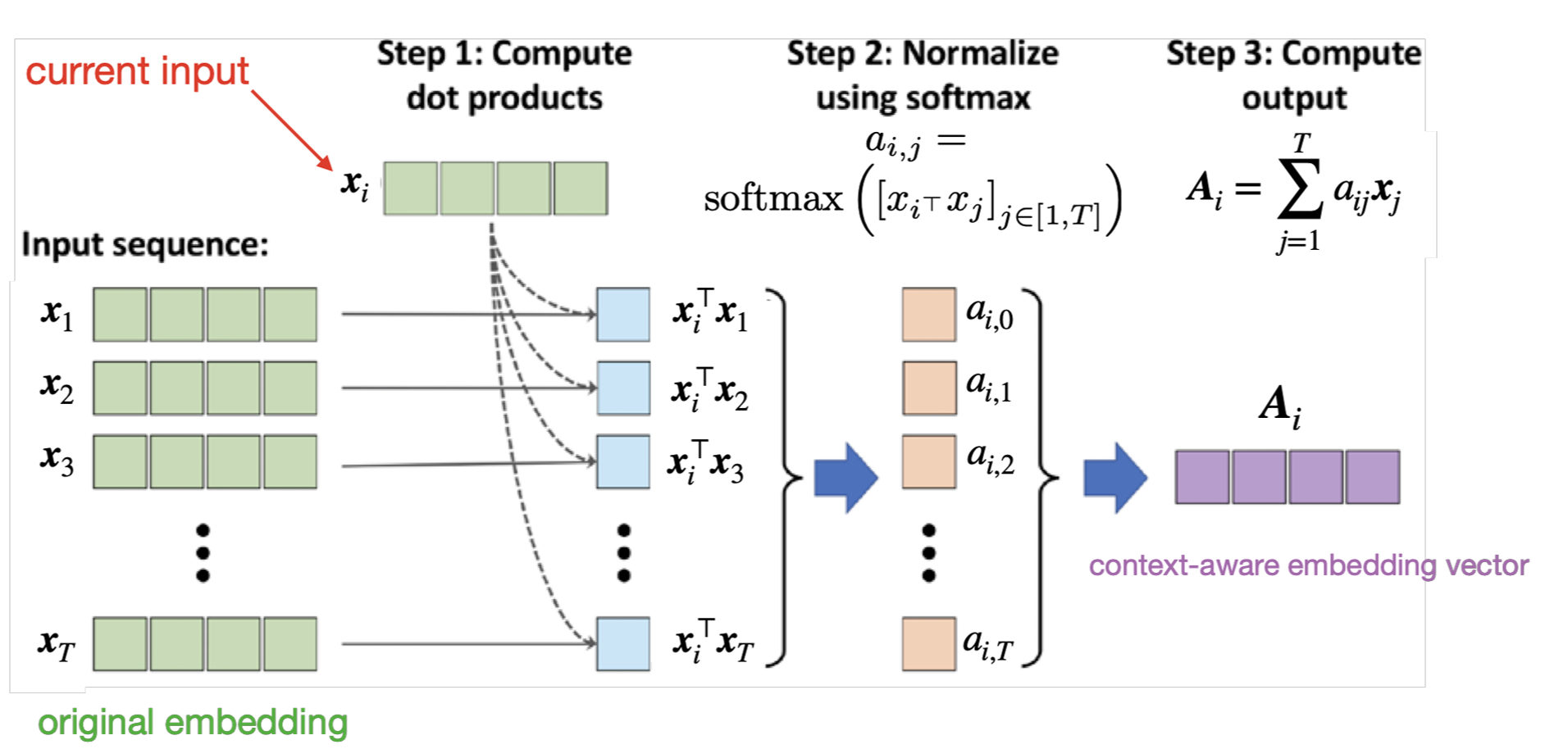
Step 1: Compute similarity scores between the current token $x_i$ and all tokens $x_j$:
This is simply the dot product between embeddings, measuring their similarity.
Step 2: Normalize scores using softmax to get attention weights:
These weights $a_{i,j}$ sum to 1 across all $j$ for each position $i$.
Step 3: Compute context-aware representation as a weighted sum:
The output $A_i$ is called a context-aware embedding vector because it incorporates information from all positions in the sequence, weighted by their relevance to position $i$.
Problem: This basic form has no learnable parameters! The model cannot learn what types of relationships to capture. The similarity is purely based on the raw embeddings.
4. Learnable Self-Attention: Query, Key, Value
(Ref: Slides 7–8)
To make self-attention learnable, we introduce three trainable weight matrices that transform the input embeddings:
where:
- $W^q \in \mathbb{R}^{d_k \times d}$ is the Query matrix
- $W^k \in \mathbb{R}^{d_k \times d}$ is the Key matrix
- $W^v \in \mathbb{R}^{d_v \times d}$ is the Value matrix
For the entire sequence, we compute:
Intuition:
- Query ($q_i$): “What am I looking for?” - Represents the information needs of position $i$
- Key ($k_j$): “What do I contain?” - Represents the content available at position $j$
- Value ($v_j$): “What information do I provide?” - The actual information to be retrieved from position $j$
Scaled Dot-Product Attention
The attention mechanism computes:
Step 1: Compute attention scores (compatibility between queries and keys):
The scaling by $\sqrt{d_k}$ prevents the dot products from becoming too large (which would cause softmax to saturate).
Step 2: Apply softmax to get attention weights:
This is a form of similarity or compatibility measure (multiplicative attention). The softmax ensures weights are normalized and can be interpreted as probabilities.
Step 3: Weighted aggregation of values:
Or in matrix form for the entire sequence:
Key Insight: For each query position $i$, the model learns which key-value pairs to attend to. The attention weights $a_{ij}$ tell us how much position $i$ should focus on position $j$.
5. Multi-Head Attention
(Ref: Slide 9)
Instead of performing attention once, Transformers use multiple attention heads operating in parallel. Each head can learn to capture different types of relationships:
The outputs of all heads are concatenated and linearly transformed:
where $W^O$ is an output projection matrix.
Benefits:
- Multiple relationship types: Different heads can specialize in different patterns (e.g., syntactic relationships, semantic relationships, positional relationships)
- Representation subspaces: Each head operates in a different representational subspace
- Rich context: The model can attend to different positions for different reasons simultaneously
Example from Slide 9: In the sentence “It is in this spirit that a majority of American governments have passed new laws since 2009 making the registration or voting process more difficult”, different attention heads capture:
- Short-range syntactic dependencies (e.g., “making” → “difficult”)
- Long-range semantic dependencies (e.g., “making” → “laws”)
- Different types of relationships shown by different colors in the visualization
6. The Complete Transformer Architecture
(Ref: Slides 10, 15–16)
The original Transformer consists of two main components:
A. Encoder Stack (Left side)
The encoder processes the entire input sequence using:
- Input Embedding: Converts tokens to dense vectors
- Positional Encoding: Adds position information (since attention is permutation-invariant)
PE*{(pos, 2i)} = \sin\left(\frac{pos}{10000^{2i/d}}\right) PE*{(pos, 2i+1)} = \cos\left(\frac{pos}{10000^{2i/d}}\right) - $N_x$ Encoder Layers, each containing:
- Multi-Head Self-Attention: Full bidirectional attention (every position can attend to every other position)
- Add & Norm: Residual connection + Layer Normalization
- Feed-Forward Network: Position-wise FFN applied independently to each position
\text{FFN}(x) = \max(0, xW_1 + b_1)W_2 + b_2 - Add & Norm: Another residual connection + Layer Normalization
Key feature: The encoder uses bidirectional (full) self-attention - each token can see all other tokens in both directions. This is optimal for understanding the input context.
B. Decoder Stack (Right side)
The decoder generates the output sequence autoregressively using:
- Output Embedding + Positional Encoding (shifted right during training)
- $N_x$ Decoder Layers, each containing:
- Masked Multi-Head Self-Attention: Causal attention that prevents positions from attending to future positions
- Uses a mask to set attention scores for future positions to $-\infty$ before softmax
- Ensures autoregressive property: position $t$ can only attend to positions $\leq t$
- Add & Norm
- Multi-Head Cross-Attention: Attends to the encoder’s output
- Queries come from the decoder
- Keys and Values come from the encoder output
- Allows decoder to focus on relevant parts of the input
- Add & Norm
- Feed-Forward Network
- Add & Norm
- Masked Multi-Head Self-Attention: Causal attention that prevents positions from attending to future positions
- Linear + Softmax: Projects to vocabulary size and produces token probabilities
Key features:
- Masked attention: Prevents information leakage from future tokens
- Cross-attention: Connects decoder to encoder for sequence-to-sequence tasks
- Autoregressive generation: Outputs one token at a time, conditioned on previous tokens
Design Principles
The Transformer architecture embodies several key principles:
- Parallelization: Unlike RNNs, all positions in a sequence can be processed simultaneously
- Residual Connections: Help with gradient flow in deep networks
- Layer Normalization: Stabilizes training
- Position-wise FFN: Adds non-linearity and increases model capacity
- Positional Encodings: Inject order information into the otherwise permutation-invariant attention
Original Use Case: The Transformer was designed for machine translation, where:
- The encoder processes the full source sentence (e.g., English)
- The decoder generates the target sentence (e.g., French) while attending to the encoded source
This encoder-decoder structure with cross-attention is ideal for tasks where you have a complete input sequence and need to generate a related output sequence.
Part 2: GPT Architecture & Probabilistic Model
(Ref: Slides 11–14, 17–21)
1. Architecture Simplification: From Transformer to GPT
GPT (Generative Pre-trained Transformer) represents a significant architectural shift from the original Transformer model.
A. The “Decoder-Only” Architecture
The original Transformer consisted of two main blocks:
- Encoder: Processes the input sequence (bidirectional attention).
- Decoder: Generates the output sequence (masked unidirectional attention) + Cross-attention to the encoder.
GPT simplifies this by removing the Encoder entirely.
- Structure: A stack of Transformer Decoder blocks.
- Removed Mechanism: The “Cross-Attention” layer (which usually connects Decoder to Encoder) is removed.
- Retained Mechanism: Masked Self-Attention.
B. Masked Self-Attention (Causal Masking)
This is the critical component that defines GPT’s behavior.
- In a standard Encoder (like BERT), a token at position $t$ can attend to all tokens ($1$ to $T$).
- In GPT (Decoder), a token at position $t$ can only attend to previous positions ($1$ to $t-1$) and itself.
- Why? To prevent “cheating” (seeing the future tokens) during the generation process.
2. Probabilistic Modeling: Next-Token Prediction
A. The Formula (Chain Rule of Probability)
Given a sequence of tokens $U = {u_1, u_2, …, u_n}$, the joint probability of the entire sequence $P(U)$ is factored using the chain rule:
$P(U) = \prod_{i=1}^{n} P(u_i \mid u_{1}, \dots, u_{i-1})$
- $u_i$: The token at the current step.
- $u_{1}, \dots, u_{i-1}$: The context window (history).
B. Training Objective
We define the loss function (typically Cross-Entropy) as:
$\mathcal{L}(\theta) = - \sum_{i} \log P(u_i \mid u_{i-k}, \dots, u_{i-1}; \theta) $
- Input: A sequence of tokens.
- Output: A probability distribution over the vocabulary for the next token.
- Process:
- Pass context through the Decoder stack.
- Output vector $h_n$ passes through a Softmax layer.
- Sample or select the highest probability token.
C. Directed Probabilistic Graphical Model
GPT can be viewed as a directed PGM:
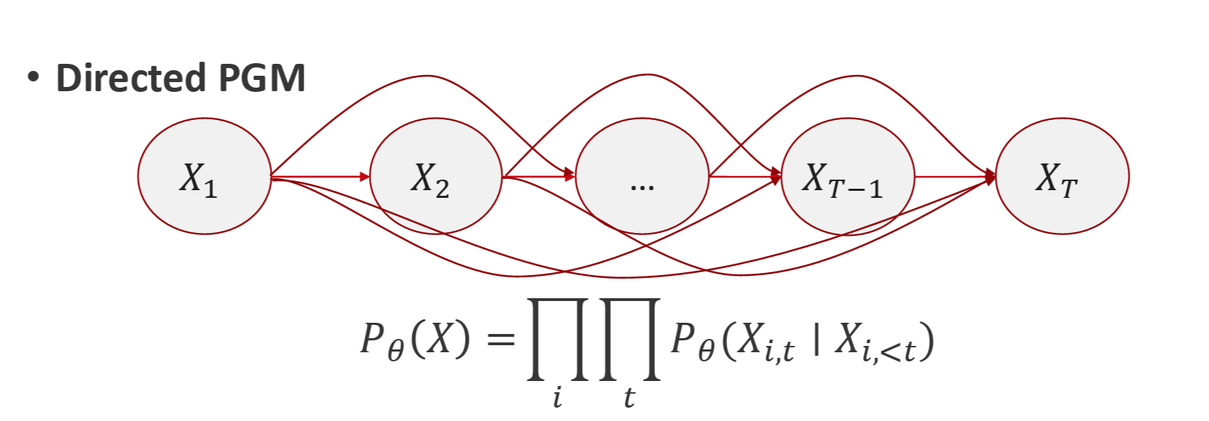
$P_{\theta}(X) = \prod_i \prod_t P_{\theta} (X_{i,t} \mid X_{i,<t})$
when we transform this probability into log-likelihood form, the probabilistic objective becomes maximizing :
$\max_{\theta} \sum_{i} \sum_{t} \log P_{\theta} (X_{i,t} \mid X_{i,<t})$
which corresponds to MLE objective.
Model structure:
- Input: token embeddings + positional encodings
- Masked multi-head attention: Enforces “causality”
- Decoder stack: Learns \(P(X_t \mid X_{<t})\)
- Output: softmax over vocabulary
3. GPT vs. Traditional Seq2Seq (Translation)
How does GPT differ from traditional Sequence-to-Sequence models (like the original Transformer or LSTM-based translation models)?
A. Traditional Seq2Seq (Encoder-Decoder)
Used typically for translation ($English \rightarrow French$).
- Mechanism:
- Encode: Read the entire English sentence into a context vector ($Context$).
- Decode: Generate French based on $p(\text{French} \mid \text{Context})$
- Key Feature: The Encoder is bidirectional (it sees the whole English sentence at once).
B. GPT (Autoregressive Language Model)
GPT does not have a separate “source” encoding stage. It treats Translation as Conditioned Generation.
- Input: It concatenates the source and the prompt into a single sequence.
- Example: “Translate to French: Hello world ->”
- Mechanism: The model predicts the next token sequentially.
- Key Difference:
- No Architecture Change: The same architecture used for writing poems is used for translation.
- Unidirectional Context: Even when reading the source sentence, GPT processes it left-to-right (though for the source part, this is less efficient than bidirectional encoding, scale compensates for it).
Summary Table
| Feature | Traditional Seq2Seq (e.g., T5) | GPT (Decoder-Only) |
|---|---|---|
| Architecture | Encoder-Decoder | Decoder-Only |
| Attention | Bidirectional (Enc) & Causal (Dec) | Causal (Masked) Only |
| Objective | Masked Language Modeling / Translation | Next-Token Prediction |
| Task Approach | Task-specific fine-tuning structure | Few-shot prompting (Input concatenation) |
Part 3: The Evolution of the GPT Series (GPT-1 to GPT-4)
(Ref: Slides 22–26, 36)
1. From our “GPT-0” to GPT-1
(Ref: Slide 23)
Moving from a simple character-level GPT to GPT-1 involves several key improvements:
Architecture Changes:
- Tokenizer: Characters → Byte-Pair Encoding (BPE) tokenizer
- More efficient representation of text
- Vocabulary of 40,000 tokens vs. 65 characters
- Activation: ReLU → GELU (Gaussian Error Linear Unit)
- Weight sharing for embedding and output layers
Scale (117M parameters):
- Layers: 4 → 12
- Attention Heads: 4 → 12
- Block size (max context): 32 → 512
- Vocab: 65 → 40,000 BPE tokens
- Embedding dim: 64 → 768
Training:
- Dataset: TinyShakespeare (1MB) → BookCorpus (5GB)
- Initialization & normalization: Default → Carefully tuned
- Optimizer: Vanilla Adam → Adam + learning rate warmup + weight decay
Inference:
- Sampling: Greedy → Top-k sampling
2. From GPT-1 to GPT-2
(Ref: Slide 24)
GPT-2 demonstrated that language models could be “unsupervised multitask learners.”
Architecture:
Scale options, with largest model at 1.5B parameters:
- Layers: 12 → 48
- Attention Heads: 12 → 25
- Embedding Dim: 768 → 1,600
- Block size (max context): 512 → 1,024
- Vocab: 40k → 50k tokens
Training:
- Dataset: BookCorpus (5GB) → WebText (40GB)
- Scraped from Reddit outbound links
- Higher quality and diversity
Note: You can reproduce GPT-2 yourself using Andrej Karpathy’s nanoGPT (takes 4 days on an 8xA100 machine)
3. From GPT-2 to GPT-3
(Ref: Slide 25)
GPT-3 demonstrated that with sufficient scale, language models become “few-shot learners.”
Architecture:
Massive scale increase to 175B parameters:
- Block size (max context): 1,024 → 2,048
- Layers: 48 → 96
- Embedding Dim: 1,600 → 12,288
- Attention Heads: 25 → 96
Training:
- Dataset: WebText (40GB) → Common Crawl + books, Wikipedia, code (~570GB)
- Significantly more diverse training data
- Better quality filtering
Key Innovation: Few-shot and zero-shot learning capabilities emerge at scale
4. From GPT-3 to GPT-4
(Ref: Slide 26)
GPT-4 represents a leap in capabilities with architectural innovations and alignment improvements.
Architecture:
- Likely includes Mixture of Experts (MoE)
- Tokenizer: Includes image patches for multimodality
- Can process both text and images
- Vision encoder integrated into the model
Scale:
- Total parameters: 175B → Likely >1T (trillion)
- Though not all parameters active per token (if using MoE)
- Block size (max context): 2,048 → 128K tokens
- Can process much longer documents
Training:
- Dataset: ~570GB → Larger, undisclosed (~50TB, 13T tokens reported)
- Alignment: Reinforcement Learning from Human Feedback (RLHF)
- Human labelers rank model outputs
- Reward model trained on preferences
- Policy fine-tuned using PPO (Proximal Policy Optimization)
- System-level “safety” measures
5. Comparison Table: GPT-1 to GPT-4
| Model | Number of parameters | Training data | Context window | Tokenizer | Architecture | New capabilities |
|---|---|---|---|---|---|---|
| GPT-1 | 117M | 5GB | 512 | BPE | Layers: 12 Heads: 12 Emb dim: 768 Vocab: 40K |
Transfer learning |
| GPT-2 | 1.5B | 40GB | 1024 | BPE | Layers: 48 Heads: 25 Emb dim: 1600 Vocab: 50K |
Zero-shot learning |
| GPT-3 | 175B | ~570GB | 2048 | BPE | Layers: 96 Heads: 96 Emb dim: 12288 Vocab: >50K |
Few-shot learning |
| GPT-4 | Likely >1T | ~50TB | 128K | Text + image patches | MoE (likely) • Larger scale (depth/width) |
• RLHF • Multimodal • Long-context reasoning |
Key Trends:
- Exponential growth in parameters and training data
- Increasing context window size
- Improved alignment and safety
- Multimodal capabilities
Part 4: Mixture of Experts (MoE) & Final Summary
(Ref: Slides 27–35)
1. Mixture of Experts (MoE): Architecture

As models scale (e.g., GPT-4), Mixture of Experts (MoE) decouples total model capacity from computational cost, allowing for massive parameter counts without slowing down inference.
A. The Core Idea

- The Experts: The standard dense Feed-Forward Network (FFNN) is replaced by multiple independent networks called “experts.”
- The Router: A learned gating mechanism that selects only the most relevant expert(s) to process a specific token.
B. Dense vs. Sparse Models
Dense Model:
- Every input activates all parameters
- High compute cost: All FFN weights are used for every token
Sparse Model (MoE):
- Uses conditional computation
- Only a small subset of parameters (e.g., 2 out of 16 experts) is activated per token
- Key advantage: Maintains fast inference despite high total capacity
C. MoE in Transformer Decoder
The FFNN layer in each Transformer block is replaced with multiple expert FFNNs:
 Dense Decoder:
Layer Norm → Masked Self-Attention → Add & Norm →
Layer Norm → [FFNN] → Add & Norm
Sparse Decoder (MoE):
Layer Norm → Masked Self-Attention → Add & Norm →
Layer Norm → [Router → Select Experts → FFNN₁, FFNN₂, ..., FFNNₙ] → Add & Norm
The router computes:
where $g_i(x)$ is the gating weight for expert $i$.
2. Probabilistic View of MoE
MoE acts as a probabilistic ensemble where the contribution of each expert is dynamic. The output probability $P(Y \mid X)$ is:
where:
- $P(Y \mid X)$ is expert $m$’s prediction
- $g_m(X)$ is the gating function (weight for expert $m$)
Constraints:
This formulation unifies several ensemble approaches:
Comparison with Other Ensemble Methods:
| Method | Gating Function $g_m(X)$ | Description |
|---|---|---|
| Bagging | $g_m(X) = \frac{1}{M}$ | Constant, uniform weighting across all experts |
| Boosting | $g_m(X) = \alpha_m$ | Constant but expert-specific weights |
| MoE | $g_m(X) = \text{Router}(X)$ | Learned function of the input - adapts per example |
Key Insight: In MoE, the gating function $g_m(X)$ is input-dependent. The model learns to route specific types of inputs to specific experts, enabling specialization.
3. Error Analysis: The Role of Diversity
The goal of MoE is to minimize the Ensemble Error rather than the individual Average Expert Error.
A. Error Definitions
Define:
- Ensemble mean: $\bar{f}(x) = \mathbb{E}[Y \mid X] = \sum_m g_m(X)\, f_m(x)$
- Individual expert mean: $f_m(x) = \mathbb{E}_m[Y \mid X]$
Compare:
- Ensemble error: $\epsilon(x) = (Y - \bar{f}(x))^2$
- Average expert error: $\bar{\epsilon}(x) = \frac{1}{M}\sum_m (Y - f_m(x))^2$
B. Analysis for Linear Models
For linear experts $f_m$, we can decompose the errors:

Key Observations:
- Ensemble error decreases with diversity (solid line, lower)
- Average expert error increases with diversity (solid line, upper)
- Disagreement between experts (dashed line) increases with diversity
Intuition: Expert errors are wrong in individualized ways and cancel out through consensus.
→ Slight “overfitting” of experts helps!
Experts that specialize (even overfit) to different data subsets create diversity, which reduces ensemble error even if individual expert errors are higher.
4. Implications for LLMs
A. Training Implications
From the error analysis, we learn:
- Encourage specialization: Experts should learn different patterns
- Load balancing challenges: Need to ensure all experts are utilized
- If one expert dominates, we lose diversity benefits
- Auxiliary losses encourage balanced expert usage
Common training challenge: Experts can collapse to similar solutions, reducing diversity.
Solutions include:
- Load balancing losses
- Expert capacity constraints
- Noise injection in routing
B. Serving Implications
 Shows the router network selecting experts and the gating mechanism for combining expert outputs.
Benefits:
- Faster inference: Only activate k out of N experts per token
- Higher capacity: Can have 10x more total parameters with similar compute
- Example: Activate 2 experts out of 16 → only ~12.5% of expert parameters used per token
Challenges:
- Memory requirements: All expert parameters must be loaded
- Load balancing: Some experts may become overloaded
- Communication overhead: In distributed settings, routing to different experts requires coordination
5. Summary: Transformer vs. GPT
While GPT originates from the Transformer architecture, it evolved specifically for generative tasks.
| Component | Original Transformer (Vaswani et al., 2017) | GPT (Generative Pre-Trained Transformer) |
|---|---|---|
| Architecture | Encoder-Decoder (Full sequence transduction) | Decoder-only (Unconditional generation) |
| Attention | Full self-attention (Bidirectional in encoder) | Masked (Causal) self-attention |
| Positional Encoding | Sinusoidal (Fixed function) | Learned positional embeddings (GPT-1+) |
| Output | Task-specific (e.g., translation) | Next-token prediction (Softmax) |
| Training Objective | Flexible / Supervised (task-specific) | Language Modeling (Autoregressive) |
| Inference | Processes full input, generates full output | Greedy / Sampling (Token-by-token) |
| Use Case | Machine translation, seq2seq tasks | Text generation, few-shot learning |
6. Summary: From GPT-1 to GPT-4
The evolution of GPT models shows consistent trends:
Architectural Evolution:
- Scale: 117M params → >1T params (10,000x increase)
- Context: 512 tokens → 128K tokens (250x increase)
- Layers: 12 → >96
- Attention Heads: 12 → >96
- Embedding Dimension: 768 → >12,288
Data Evolution:
- Size: 5GB → ~50TB (10,000x increase)
- Quality: BookCorpus → Curated web + books + code
- Diversity: Single domain → Multi-domain, multi-modal
Capability Evolution:
- GPT-1: Transfer learning via fine-tuning
- GPT-2: Zero-shot task generalization
- GPT-3: Few-shot in-context learning
- GPT-4: Multimodal understanding, enhanced reasoning, RLHF alignment
Architectural Innovations:
- Tokenization: Character → BPE → Enhanced BPE + image patches
- Activation: ReLU → GELU
- Sparse Architectures: Dense FFN → Mixture of Experts (likely in GPT-4)
- Alignment: Pure language modeling → RLHF for human preference alignment
Conclusion
This lecture traced the evolution from RNNs through Transformers to modern GPT architectures:
- RNNs had fundamental limitations in parallelization and long-range dependencies
- Transformers solved these with self-attention and parallel processing
- GPT simplified the Transformer to a decoder-only architecture focused on language modeling
- Scaling from GPT-1 to GPT-4 showed that increased capacity, data, and training enable emergent capabilities
- Mixture of Experts enables continued scaling by decoupling model capacity from computational cost
The key insights are:
- Attention is all you need for sequence modeling
- Causal masking enables autoregressive generation
- Scale (parameters, data, compute) unlocks qualitatively new capabilities
- Sparse architectures like MoE allow continued scaling
- Alignment through RLHF is crucial for deploying powerful models safely
References
-
Vaswani, A., Shazeer, N., Parmar, N., Uszkoreit, J., Jones, L., Gomez, A.N., Kaiser, L. and Polosukhin, I., 2017. Attention Is All You Need. NeurIPS 2017.
-
Radford, A., Narasimhan, K., Salimans, T. and Sutskever, I., 2018. Improving Language Understanding by Generative Pre-Training. OpenAI.
-
Radford, A., Wu, J., Child, R., Luan, D., Amodei, D. and Sutskever, I., 2019. Language Models are Unsupervised Multitask Learners. OpenAI.
-
Brown, T., Mann, B., Ryder, N., et al., 2020. Language Models are Few-Shot Learners. NeurIPS 2020.
-
OpenAI, 2023. GPT-4 Technical Report.
-
Jacobs, R.A., Jordan, M.I., Nowlan, S.J. and Hinton, G.E., 1991. Adaptive Mixtures of Local Experts. Neural Computation.
-
Jordan, M.I. and Jacobs, R.A., 1994. Hierarchical Mixtures of Experts and the EM Algorithm. Neural Computation.
-
Shazeer, N., et al., 2017. Outrageously Large Neural Networks: The Sparsely-Gated Mixture-of-Experts Layer. ICLR 2017.
-
Sollich, P. and Krogh, A., 1995. Learning with Ensembles: How Overfitting Can Be Useful. NeurIPS 1995.
-
Yang, L., et al., 2023. A Survey on Transformers. arXiv preprint.
-
Grootendorst, M., A Visual Guide to Mixture of Experts. Blog post.
-
Xie, S., et al., 2022. On the Role of the Action Space in Robot Manipulation Learning. arXiv preprint.